ZooScan image segmentation using a UNet with a pretrained backbone
%load_ext autoreload
%autoreload 2
In this lab, we would like to train a deep neural network for performing semantic segmentation of Zooscan images. This labwork will guide through :
- how to load labeled zooscan images
- how to implement a UNet for performing the semantic segmentation
- how to train the network
- how to perform inference on a new image with a trained network
The cell below will collect a subset of a dataset for training and testing. The complete dataset we can use is made of $23$ labeled zooplankton images provided by :
Sorbonne Université/CNRS - Institut de la Mer de Villefranche (IMEV), Sorbonne Université/CNRS - Laboratoire d'Océanographie de Villefranche (LOV); 2020; Plankton community in Régent (680µm) net, Point B, Villefranche-sur-Mer, France https://dx.doi.org/10.14284/477
!rm -rf data
import os
import glob
import random
import shutil

max_numfiles = 10
train_fraction = 0.8

datarootdir = "/mounts/Datasets3/2024-2025-ChallengePlankton/train"

if "TMPDIR" in os.environ:
    # On the DCE, $TMPDIR refer to a temporary local storage on the compute node
    tmpdir = os.environ["TMPDIR"]
    os.symlink(tmpdir, "./data")
else:
    tmpdir = "./data"

if os.path.exists(tmpdir):
    shutil.rmtree(tmpdir)

os.makedirs(tmpdir)

# Locate all the xxxxx_scan.png.ppm from the datarootdir with the labels xxxxx_mask.png.ppm
# split it randomly in 80% train and 20% test
# Only consider up to max_numfiles files
# Copy these data in their respective folders into the tmpdir

scan_files = glob.glob(os.path.join(datarootdir, "*_scan.png.ppm"))
# Compute the mask filenames from the scan files
mask_files = [f.replace("_scan.png.ppm", "_mask.png.ppm") for f in scan_files]

# Random shuffle the files for the split. Apply the same random to the masks to keep
# both lists aligned

idx = list(range(len(scan_files)))[:max_numfiles]
random.shuffle(idx)

train_idx = idx[: int(len(idx) * train_fraction)]
test_idx = idx[int(len(idx) * train_fraction) :]

train_scan_files = [scan_files[i] for i in train_idx]
train_mask_files = [mask_files[i] for i in train_idx]
test_scan_files = [scan_files[i] for i in test_idx]
test_mask_files = [mask_files[i] for i in test_idx]


def copy_files(files, target_dir):
    """
    Copy the files to the target directory.
    """
    if not os.path.exists(target_dir):
        os.makedirs(target_dir)
    for f in files:
        os.system(f"cp {f} {target_dir}")


# Copy the files to the tmpdir
copy_files(train_scan_files, os.path.join(tmpdir, "train"))
copy_files(train_mask_files, os.path.join(tmpdir, "train"))

copy_files(test_scan_files, os.path.join(tmpdir, "test"))
copy_files(test_mask_files, os.path.join(tmpdir, "test"))

# Copy the taxa file as well
os.system(f"cp {datarootdir}/taxa.csv {os.path.join(tmpdir, 'train')}")
os.system(f"cp {datarootdir}/taxa.csv {os.path.join(tmpdir, 'test')}")
0
Introduction
We are provided with labeled zooscan which means we have both the zooscan image and a mask. The mask is an image of labels. The data are located within the data subdirectory; Every scan is around $20000\times 15000$ pixels.
!ls data/train
rg20090204_mask.png.ppm  rg20090617_mask.png.ppm  rg20091028_mask.png.ppm
rg20090204_scan.png.ppm  rg20090617_scan.png.ppm  rg20091028_scan.png.ppm
rg20090318_mask.png.ppm  rg20090715_mask.png.ppm  rg20091125_mask.png.ppm
rg20090318_scan.png.ppm  rg20090715_scan.png.ppm  rg20091125_scan.png.ppm
rg20090610_mask.png.ppm  rg20090902_mask.png.ppm  taxa.csv
rg20090610_scan.png.ppm  rg20090902_scan.png.ppm
!for f in data/train/*_scan.png.ppm; do file $f; done
data/train/rg20090204_scan.png.ppm: Netpbm image data, size = 22817 x 14569, rawbits, greymap
data/train/rg20090318_scan.png.ppm: Netpbm image data, size = 22797 x 14549, rawbits, greymap
data/train/rg20090610_scan.png.ppm: Netpbm image data, size = 22717 x 14459, rawbits, greymap
data/train/rg20090617_scan.png.ppm: Netpbm image data, size = 22817 x 14529, rawbits, greymap
data/train/rg20090715_scan.png.ppm: Netpbm image data, size = 22807 x 14549, rawbits, greymap
data/train/rg20090902_scan.png.ppm: Netpbm image data, size = 22807 x 14319, rawbits, greymap
data/train/rg20091028_scan.png.ppm: Netpbm image data, size = 22787 x 14379, rawbits, greymap
data/train/rg20091125_scan.png.ppm: Netpbm image data, size = 22817 x 14519, rawbits, greymap
An example ZooScan image and its mask are displayed below
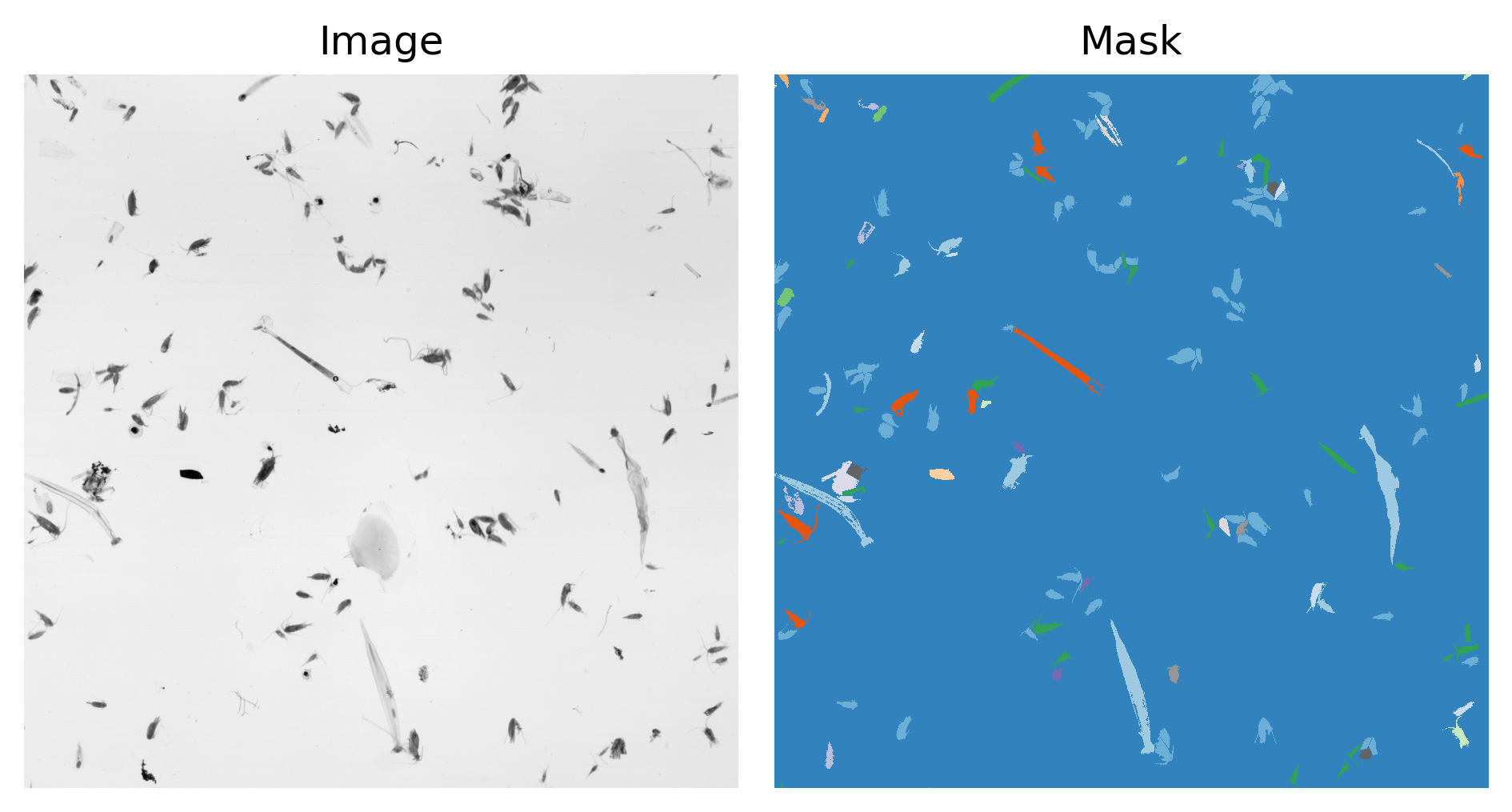
The colorcode of the mask is dependent on the class to which the pixel has been assigned by the human labeler Note this is certainly a tough work to pixel label these huge images but the quality of your data and labels are of the uppermost importance for our deep learning algorithms to work. The semantic of the class indices are provided in the taxa.csv file.
!cat data/train/taxa.csv
label,living,label_nb
artefact,False,1
badfocus<artefact,False,2
bubble,False,3
detritus,False,4
fiber<detritus,False,5
t001,False,6
t003,False,7
Abylopsis tetragona,True,8
Acartiidae,True,9
Actiniaria,True,10
Actinopterygii,True,11
Aglaura,True,12
Amphipoda,True,13
Annelida,True,14
Atlanta,True,15
Aulacantha,True,16
Bivalvia<Mollusca,True,17
Calanidae,True,18
Calanoida,True,19
Calocalanus pavo,True,20
Candaciidae,True,21
Cavolinia inflexa,True,22
Centropagidae,True,23
Chaetognatha,True,24
Chelophyes appendiculata,True,25
Cliidae,True,26
Collodaria,True,27
Copilia,True,28
Corycaeidae,True,29
Creseidae,True,30
Creseis acicula,True,31
Ctenophora<Metazoa,True,32
Cymbulia peroni,True,33
Doliolida,True,34
Echinodermata,True,35
Eucalanidae,True,36
Euchaetidae,True,37
Eumalacostraca,True,38
Evadne,True,39
Fritillariidae,True,40
Gammaridea,True,41
Globigerinidae,True,42
Gymnosomata,True,43
Haloptilus,True,44
Harpacticoida,True,45
Heterorhabdidae,True,46
Hydrozoa,True,47
Hyperiidea,True,48
Insecta,True,49
Lensia subtilis,True,50
Limacinidae,True,51
Liriope<Geryoniidae,True,52
Metridinidae,True,53
Mollusca,True,54
Obelia,True,55
Oikopleuridae,True,56
Oithonidae,True,57
Oncaeidae,True,58
Orbulina,True,59
Ostracoda,True,60
Penilia avirostris,True,61
Physonectae,True,62
Podon,True,63
Pontellidae,True,64
Pontellina plumata,True,65
Pyrosomatida,True,66
Rhincalanidae,True,67
Rhizaria,True,68
Rhopalonema velatum,True,69
Salpida,True,70
Sapphirinidae,True,71
Solmundella bitentaculata,True,72
Temoridae,True,73
bract<Abylidae,True,74
bract<Abylopsis tetragona,True,75
bract<Diphyidae,True,76
calyptopsis<Euphausiacea,True,77
chain<Salpida,True,78
cirrus,True,79
colony<Phaeodaria,True,80
cypris,True,81
damaged<Aulacantha,True,82
division,True,83
egg<Actinopterygii,True,84
egg<Mollusca,True,85
egg<other,True,86
ephyra<Scyphozoa,True,87
eudoxie<Abylopsis tetragona,True,88
eudoxie<Bassia bassensis,True,89
eudoxie<Diphyidae,True,90
gonophore<Abylopsis tetragona,True,91
gonophore<Bassia bassensis,True,92
gonophore<Diphyidae,True,93
head<Chaetognatha,True,94
juvenile<Salpida,True,95
larvae<Annelida,True,96
larvae<Porcellanidae,True,97
larvae<Squillidae,True,98
like<Collodaria,True,99
like<Laomediidae,True,100
megalopa,True,101
multiple<Copepoda,True,102
multiple<other,True,103
nauplii<Cirripedia,True,104
nauplii<Crustacea,True,105
nectophore<Abylopsis tetragona,True,106
nectophore<Bassia bassensis,True,107
nectophore<Diphyidae,True,108
nectophore<Hippopodiidae,True,109
nectophore<Physonectae,True,110
nucleus<Salpidae,True,111
othertocheck,True,112
part<Annelida,True,113
part<Cnidaria,True,114
part<Crustacea,True,115
part<Ctenophora,True,116
part<Mollusca,True,117
part<Siphonophorae,True,118
phyllosoma,True,119
pluteus<Echinoidea,True,120
pluteus<Ophiuroidea,True,121
protozoea<Mysida,True,122
protozoea<Penaeidae,True,123
protozoea<Sergestidae,True,124
scale,True,125
seaweed,True,126
siphonula,True,127
t002,True,128
tail<Appendicularia,True,129
tail<Chaetognatha,True,130
trunk<Appendicularia,True,131
wing,True,132
zoea<Brachyura,True,133
zoea<Galatheidae,True,134
We do have $134$ classes of objects plus the background (label $0$). All the living stuff have been assigned a label strictly higher than $7$. The "living" column is exactly the same as testing if the label_nb is smaller or larger than $7$.
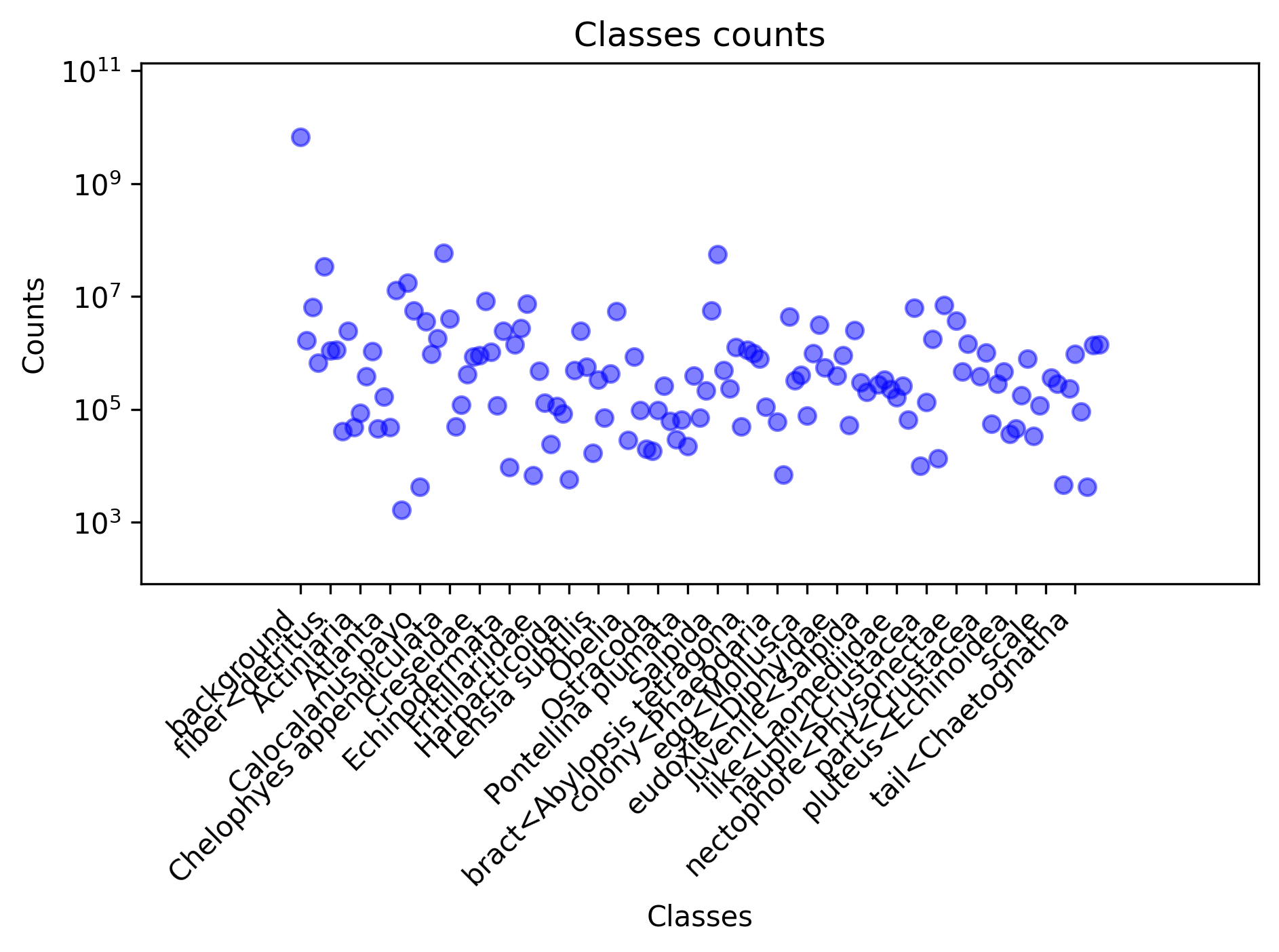
The classes are unbalanced. For example, counting the number of occurences of all the $135$ classes (background + $134$ non living stuff and living organisms), we obtain the count below, by decreasing occurence.
The most represented class is the background with almost $6$ billions pixels. The most represented non-background class is Chaetognatha (class label $50$) with $58$ million pixels and the less represented class is Bivalvia/Mollusca with only $1163$ K pixels. This strong unbalance can induce a lot of trouble when training a neural network as the over-represented classes can be more easily learned than the under-represented ones.
| Classe name | Count |
|---|---|
| background | 6648643689 |
| Chaetognatha | 58412864 |
| Salpida | 56586684 |
| detritus | 33649190 |
| Calanidae | 17664122 |
| Aulacantha | 12856260 |
| Creseis acicula | 8225786 |
| Eumalacostraca | 7416376 |
| nectophore<Diphyidae | 7036773 |
| badfocus<artefact | 6540988 |
| multiple<other | 6236479 |
| Rhopalonema velatum | 5682772 |
| Calanoida | 5602157 |
| Metridinidae | 5429665 |
| damaged<Aulacantha | 4346996 |
| Chelophyes appendiculata | 4061841 |
| nectophore<Physonectae | 3743692 |
| Candaciidae | 3646939 |
| ephyra<Scyphozoa | 3104710 |
| Euchaetidae | 2741439 |
| gonophore<Diphyidae | 2502463 |
| Abylopsis tetragona | 2443476 |
| Doliolida | 2442549 |
| Hydrozoa | 2418177 |
| Centropagidae | 1803662 |
| nectophore<Abylopsis tetragona | 1760329 |
| artefact | 1672201 |
| othertocheck | 1434265 |
| zoea<Galatheidae | 1407337 |
| Eucalanidae | 1393273 |
| zoea<Brachyura | 1360657 |
| Temoridae | 1258350 |
| t001 | 1142346 |
| bract<Abylopsis tetragona | 1135173 |
| fiber<detritus | 1094546 |
| Aglaura | 1071800 |
| Ctenophora<Metazoa | 1046977 |
| part<Crustacea | 999993 |
| egg<other | 995258 |
| bract<Diphyidae | 991480 |
| Cavolinia inflexa | 954769 |
| tail<Chaetognatha | 951886 |
| Creseidae | 914248 |
| gonophore<Abylopsis tetragona | 908079 |
| Corycaeidae | 853293 |
| Oikopleuridae | 846252 |
| protozoea<Mysida | 780997 |
| calyptopsis<Euphausiacea | 780051 |
| bubble | 659786 |
| Hyperiidea | 570687 |
| eudoxie<Abylopsis tetragona | 548613 |
| Sapphirinidae | 490605 |
| Heterorhabdidae | 487610 |
| Fritillariidae | 481907 |
| nucleus<Salpidae | 468802 |
| part<Siphonophorae | 461031 |
| Liriope<Geryoniidae | 428388 |
| Copilia | 413538 |
| egg<Actinopterygii | 400252 |
| Pyrosomatida | 393117 |
| eudoxie<Diphyidae | 391068 |
| Actinopterygii | 386618 |
| part<Cnidaria | 380051 |
| seaweed | 361969 |
| Lensia subtilis | 331479 |
| larvae<Squillidae | 329856 |
| division | 326004 |
| head<Chaetognatha | 299446 |
| siphonula | 286749 |
| part<Mollusca | 285145 |
| larvae<Porcellanidae | 278677 |
| megalopa | 259496 |
| Penilia avirostris | 259458 |
| tail<Appendicularia | 234629 |
| Solmundella bitentaculata | 232568 |
| like<Collodaria | 224458 |
| Rhizaria | 217177 |
| juvenile<Salpida | 201881 |
| pluteus<Ophiuroidea | 178319 |
| Annelida | 166785 |
| like<Laomediidae | 164274 |
| nauplii<Crustacea | 133174 |
| Gammaridea | 131295 |
| Collodaria | 118535 |
| Cymbulia peroni | 117545 |
| protozoea<Sergestidae | 115471 |
| Gymnosomata | 114724 |
| chain<Salpida | 109933 |
| Oithonidae | 96581 |
| Ostracoda | 96258 |
| trunk<Appendicularia | 91666 |
| Actiniaria | 86592 |
| Haloptilus | 84510 |
| egg<Mollusca | 76979 |
| Limacinidae | 70271 |
| Rhincalanidae | 70044 |
| Pontellidae | 65340 |
| multiple<Copepoda | 64726 |
| Physonectae | 61635 |
| colony<Phaeodaria | 60429 |
| part<Ctenophora | 55696 |
| gonophore<Bassia bassensis | 51563 |
| bract<Abylidae | 50050 |
| Cliidae | 49886 |
| Atlanta | 48107 |
| Acartiidae | 47749 |
| Amphipoda | 45436 |
| pluteus<Echinoidea | 45399 |
| t003 | 40408 |
| phyllosoma | 36785 |
| protozoea<Penaeidae | 33334 |
| Podon | 29154 |
| Obelia | 28436 |
| Globigerinidae | 24077 |
| Pontellina plumata | 22435 |
| Oncaeidae | 20112 |
| Orbulina | 18316 |
| Insecta | 16989 |
| nectophore<Bassia bassensis | 13441 |
| nauplii<Cirripedia | 9843 |
| Echinodermata | 9496 |
| cypris | 6894 |
| Evadne | 6758 |
| Harpacticoida | 5712 |
| t002 | 4580 |
| Calocalanus pavo | 4258 |
| wing | 4236 |
| Bivalvia<Mollusca | 1663 |
| eudoxie<Bassia bassensis | 0 |
| cirrus | 0 |
| larvae<Annelida | 0 |
| part<Annelida | 0 |
| scale | 0 |
| nectophore<Hippopodiidae | 0 |
| Mollusca | 0 |
The plot below shows the number of pixels per class. Note that the y-axis is in logscale. As we count the number of pixels per class, the unbalance could be explained by some organisms larger than others or by the over-representation of these. In any case, this unbalance will cause you trouble when training a neural network.
If we group the classes by non-living vs living, we obtain the following counts where you still have $10$ times more "non living pixels".
| Classe name | Count |
|---|---|
| Non living | 6.693.443.154 |
| Living | 259.647.119 |
Imports
All the code you are going to write will be into the following files :
data.py: script responsible for handling the data pipeline, producing the dataloaders for the training and validation datamodels/: submodule responsible for providing the different models you want to experiment
# Standard imports
import pathlib

# External imports
import albumentations as A
import numpy as np
import matplotlib.pyplot as plt
import torch
import yaml

# Local imports
import wandb
import planktoseg
from planktoseg import data
from planktoseg import models
from planktoseg import optim
from planktoseg import utils
from planktoseg import metrics
from planktoseg import main

use_cuda = torch.cuda.is_available()
device = torch.device("cuda") if use_cuda else torch.device("cpu")

logdir = pathlib.Path("./logs")
if not logdir.exists():
    logdir.mkdir(exist_ok=True)
/usr/users/dce-admin/fix/GIT/2024_ml4oceans/venv/lib/python3.10/site-packages/requests/__init__.py:86: RequestsDependencyWarning: Unable to find acceptable character detection dependency (chardet or charset_normalizer).
  warnings.warn(
Data loading and exploration
In this part, we will be exploring the dataset :
- load and visualize some samples
- investigate the balance of the classes
- investigate the application of some data augmentation techniques.
The very first step when you write a pipeline for training neural networks on your data is to prepare your data pipeline.
In Pytorch, the expected output of this first step is to provide the data loaders, i.e. the python iterable objects able to give you minibatches for training and validation.
Dataset
In the data.py script, you are provided with the PlanktonDataset object. We wrote this class to ease your work of loading the data. This class can :
- load the data (image and mask),
- split every sample into patches and you can configure both the patch size and the patch stride (overlap = patch_size - patch_stride),
- apply transformations on the input patches and mask patches
- switch between two semantic segmentation tasks :
- classify a pixel as belonging to one of the $135$ classes (
task = SegmentationTask.LIVING_CLASSES) - classify a pixel as belonging to non living vs living classes (
task = SegmentationTask.LIVING_NONLIVING)
- classify a pixel as belonging to one of the $135$ classes (
As an example, in the cell below, we basically invoke this dataset object which is going to :
- split the large scans into patches of size $512 \times 512$ with a stride of $128 \times 128$
- merge the labels into two classes : Non living (label < 7) and Living (label >= 8)
- every patch and mask are transformed from an Image type to pytorch Tensor
transform = A.pytorch.ToTensorV2()

dataset = data.PlanktonDataset(root="./data/train", patch_size=(512, 512), patch_stride=(128, 128), task=data.SegmentationTask.LIVING_NONLIVING)
dataset = data.WrappedDataset(dataset, transform)
100%|██████████| 8/8 [00:00<00:00, 7584.64it/s]
100%|██████████| 8/8 [00:00<00:00, 7584.64it/s]
We can now access both an image and its label by indexing the dataset. Feel free to repeat the execution of the cell below as it randomly samples the dataset for a new image/mask.
Feel free to run the cell below multiple times. Every time, it will randomly sample one patch and its binary label.
idx = np.random.randint(len(dataset))

img, mask = dataset[idx]

print(f"The img is of type {type(img)} and of shape {img.shape}")
print(f"The mask is of type {type(mask)} and of shape {mask.shape}")

plt.subplot(1, 2, 1)
plt.imshow(img.squeeze(), cmap="gray")
plt.title("Zooscan image")
plt.axis("off")

plt.subplot(1, 2, 2)
plt.imshow(mask.squeeze(), interpolation="none", cmap="tab20c")
plt.title("Mask")
plt.axis("off")
The img is of type <class 'torch.Tensor'> and of shape torch.Size([1, 512, 512])
The mask is of type <class 'torch.Tensor'> and of shape torch.Size([512, 512])
(np.float64(-0.5), np.float64(511.5), np.float64(511.5), np.float64(-0.5))

Exploring the augmentation transforms
Data (of quality) is of paramount importance but still limited in availability. We can virtually increase its availability by applying so called "data augmentations" which are transforms of your inputs for which you know how to transform the target.
For this, we will use the albumentations python library which offers several transforms for various tasks (classification, object detection, semantic segmentation)
Your first exercise is to identify, among the available data transforms (see for example this documentation and do not forget to scroll down to the spatial level transforms) which ones can be suitable. For example :
- A.HorizontalFlip, which randomly flips horizontally your image/mask pair,
- A.VerticalFlip which randomly flips vertically your image/mask pair,
- A.MaskDropout which randomly mask some objects
You could also Blur or add GaussianNoise. I believe these transforms still make sense for our plankton segmentation task given the snow we see on the image and the possibly un-focused objects. If you wonder about "Where should I stop adding transforms ?" / "How do I know my transforms are ok ?". Remember, the purpose of these transforms is to augment your data, hopefully to improve your validation metric. We look for transforms that will improve the ability of your neural network to generalize its responses on new images.
In the sample code below, you can experiment with different augmentations. Some are already provided, feel free to :
- run multiple times the cell below. The transforms are randomly sampled and applied on the inputs. Every time you run the cell, the same input image/mask will be differently transformed
- modify the content of the
transform = A.Compose([..])to add or remove transforms and observe its impact
idx = np.random.randint(len(dataset))
idx = 15000

# Sample the dataset without all the transforms
# to see what the image and mask originally look like
original_transform = A.pytorch.ToTensorV2()
dataset.transform = original_transform
orig_img, orig_mask = dataset[idx]

##########################################################################################
# TODO: Feel free to change the code below
# Tune the augmented transform by prepending your choosen transform before the
# conversion to pytorch tensor
# Fill free to evaluate the cell as you add transforms to see their effect
transform = A.Compose([
    A.HorizontalFlip(p=0.5),
    A.RandomRotate90(p=0.5),
    A.MaskDropout((1, 1), image_fill_value=255, p=1),
    A.Blur(),
    A.pytorch.ToTensorV2()
])
##########################################################################################

# And now sample the exact same image/mask
dataset.transform = transform
aug_img, aug_mask = dataset[idx]

plt.subplot(2, 2, 1)
plt.imshow(orig_img.squeeze(), cmap="gray", clim=(0, 255))
plt.title("Zooscan original")
plt.axis("off")

plt.subplot(2, 2, 2)
plt.imshow(orig_mask.squeeze(), interpolation="none", cmap="tab20c")
plt.title("Original Mask")
plt.axis("off")

plt.subplot(2, 2, 3)
plt.imshow(aug_img.squeeze(), cmap="gray", clim=(0, 255))
plt.title("Zooscan augmented image")
plt.axis("off")

plt.subplot(2, 2, 4)
plt.imshow(aug_mask.squeeze(), interpolation="none", cmap="tab20c")
plt.title("Augmented mask")
plt.axis("off")
/tmp/fix-108932/ipykernel_2324214/2288155435.py:18: UserWarning: Argument(s) 'image_fill_value' are not valid for transform MaskDropout
  A.MaskDropout((1, 1), image_fill_value=255, p=1),
(np.float64(-0.5), np.float64(511.5), np.float64(511.5), np.float64(-0.5))

Adding the transforms in the data pipeline
The suitable augmentation transforms you identified in the previous sections needs to be given in the data pipeline.
This is already defined in the planktoseg/data.py script. The most important function in the data.py script is the get_dataloaders function where :
- the dataset is split between a training and validation folds
- both with their own transforms (with augmentations for the training, without augmentation for the validation)
- creates the dataloaders providing the mini batches
The get_dataloaders is the function that will be called by the main script to build up the dataloaders, and that's the only thing we need from the data pipeline.
Locate in the planktoseg/data.py script, in the get_dataloaders function, where and which transforms are defined. Once done, move forward with the next cell which will create your dataloaders.
# The configuration below requires 11GB of VRAM
data_config = {"trainpath": "./data/train",
               "valid_ratio": 0.2,
               "batch_size": 32,
               "num_workers": 7,
               "patch_size": (256, 256),
               "patch_stride": (128, 128),
               "task": "living_nonliving",
               "normalize": True,
               "max_num_samples": 50000
               }

train_loader, valid_loader, input_size, num_classes, normalizing_stats = data.get_dataloaders(data_config, use_cuda)

# The normalizing statistics must be saved because they will be needed for inference
with open(logdir / "normalizing_stats.yaml", "w") as file:
    yaml.dump(normalizing_stats, file)
100%|██████████| 8/8 [00:00<00:00, 4497.91it/s]
100%|██████████| 1250/1250 [01:24<00:00, 14.83it/s]
print(f"The train dataloader contains {len(train_loader)} mini batches")
print(f"The valid dataloader contains {len(valid_loader)} mini batches")
print(f"Our problem contains {num_classes} classes and our inputs have the shape {input_size}")
print(f"For normalizing the input, we will be using the following statistics {normalizing_stats}")
The train dataloader contains 1250 mini batches
The valid dataloader contains 313 mini batches
Our problem contains 2 classes and our inputs have the shape (1, 256, 256)
For normalizing the input, we will be using the following statistics {'mean': 0.8375427017211914, 'std': 0.09082679715796328}
Encoder/Decoder with a pretrained backbone
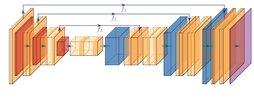
Since we now have the data to train on, the next step is to implement the model. We are going to implement a U-Net, as seen during the lecture, with a pre-trained backbone.
In our codebase, it is the responsibility of the models module to build the models. This module provides you a builder of models which is the models.build_model function. The UNet model is defined in the models/unet.py script as the UNet class. If you look at the code of that class, you will notice it is built with two components : the encoder which is a TimmEncoder and the decoder of type Decoder.
Locate in the planktoseg/models/unet.py the class TimmEncoder. This class is using the external library timm to access pretrained neural networks. In particular, an encoder has exactly the stucture of a classification network and it makes sense to use, for example, a ResNet pretrained on ImageNet as an initial encoder.
To better appreciate what the encoder produces as an output, the cell below will :
- create an encoder with
cin=1(grayscale input images) andmodel_name=resnet18 - perform a forward pass through the network and check the dimensionality of the outputs.
As we are only interested in checking the dimensionalities of the output of the encoder, you can use a dummy torch.zeros tensor to perform the forward propagation. This is handful way to trigger the computation of a network.
from planktoseg.models.unet import TimmEncoder

encoder = TimmEncoder(cin=1, model_name="resnet18")
fake_input = torch.zeros(1, 1, 512, 512) # This must be in the pytorch format (B, C, H, W)
f4, [f1, f2, f3] = encoder(fake_input)

print(f"With an input of shape {fake_input.shape}, \n our model outputs tensors of shape :")
print(f" - f1 : {f1.shape}")
print(f" - f2 : {f2.shape}")
print(f" - f3 : {f3.shape}")
print(f" - f4 : {f4.shape}")
With an input of shape torch.Size([1, 1, 512, 512]),
 our model outputs tensors of shape :
 - f1 : torch.Size([1, 64, 128, 128])
 - f2 : torch.Size([1, 128, 64, 64])
 - f3 : torch.Size([1, 256, 32, 32])
 - f4 : torch.Size([1, 512, 16, 16])
Implementing the decoder
We now move on the decoder part. The decoder receives the outputs of the encoder and progressively upscales spatially the representation to finally obtain an output whose spatial dimensions match the ones of the input, and produce, for every pixel, a score for each of our $2$ classes.
With an input of shape $(B, C, H, W)$, the output of the final layer is expected to be of shape $(B, K, H, W)$ where $K$ is the number of classes you want to predict for every pixel.
The specificity of the UNet is that along the upscaling path, you integrate features from intermediate layers of the encoder through the so-called shortcut connections, the connections that provide the $f_3, f_2, f_1$ features depicted on the figure above.
Locate the code of the Decoder class in the models.py script. As the encoder, the decoder is built from the repetition of blocks, so called DecoderBlock in the code. All the codes are already prodived to you and you can take time to understand what is going on.
A Decoder block receives, along the upscaling path, an input tensor with cin channels and is built from a sequence of layers :
conv1which is a Sequential block with 2D convolution, Batch normalization layer and ReLU. This sub-block should outputcinchannels,up_convwhich is a Sequential block with an upscaling layer followed by a 2D convolution, Batch normalization and ReLU. This sub-block should outputcin//2channelsconv2which is a sequential block with a 2D convolution, Batch normalization layer and ReLU. This sub-block takes as inputcinchannels and outputscin//2channels.
For the forward pass, your decoder block receives two inputs : x and f_encoder. The tensor x are the features that are flowing through the upscaling path while f_encoder are the features received from the encoder through the shortcut connections. During the forward pass you need to :
- pass the
xfeatures throughconv1andup_conv, - concatenate the output of the previous step with the encoder features
f_encoder, - pass the output of the previous step through the final sub-block
conv2
Note how the dimensions change during these steps. At the output of up_conv, your tensor will have cin//2 channels. The f_encoder contains cin//2 channels as well. When both are concatenated, your tensor has cin channels and the final conv2 transforms these into cin//2 channels.
To test your implementation, you can run the following cell which should complete without errors. When you code your own network, it is definitely a good practice to locally test your implementation. You want to locate potential errors as soon as possible. Imagine if you had to debug your code only when all the pipeline is setup, what a nightmare 😱 ! Just never do that !
from planktoseg.models.unet import DecoderBlock, Decoder

# First test : we check the forward pass through a decoder block is working
print("First test")
dummy_input = torch.zeros(3, 4, 128, 128)
dummy_encoder_features = torch.zeros(3, 2, 256, 256)
block = DecoderBlock(4)
output = block(dummy_input, dummy_encoder_features)

print(f"With an input of shape {dummy_input.shape} with encoder features of shape {dummy_encoder_features.shape}, the output of the decoder block is of shape {output.shape}")

assert list(output.shape) == [3, 2, 256, 256]

# Second test : we check the forward pass through a complete decoder is working
print("\nSecond test")
batch_size = 3
K = 10
f1 = torch.zeros(batch_size, 64, 128, 128)
f2 = torch.zeros(batch_size, 128, 64, 64)
f3 = torch.zeros(batch_size, 256, 32, 32)
f4 = torch.zeros(batch_size, 512, 16, 16)

decoder = Decoder(num_classes = K)
output = decoder(f4, [f1, f2, f3])

print(f"The output of the decoder is of shape {output.shape}")

assert list(output.shape) == [batch_size, K, 512, 512]
print("If we reach that point, we are good to go !")
First test
With an input of shape torch.Size([3, 4, 128, 128]) with encoder features of shape torch.Size([3, 2, 256, 256]), the output of the decoder block is of shape torch.Size([3, 2, 256, 256])

Second test
The output of the decoder is of shape torch.Size([3, 10, 512, 512])
If we reach that point, we are good to go !
Building the complete model
Once the encoder and decoder are implemented, we can create the complete model and send it to the device used for the experiments.
%%capture

model = models.UNet({"encoder": {"model_name": "resnet18"}}, input_size, 1 if num_classes == 2 else num_classes)
model = model.to(device)
Loss function and metrics for an unbalanced classification
Great, we have the data and we have a model. It is now time to define the loss which quantifies the mismatch between the predictions of our network and the groundtruth, and the metrics which will help us monitor the training.
Our problem is a classification problem, although pixel-wise. You need to classify every single pixel of an image. A natural first guess loss function in this case in the cross entropy loss which reads :
$$ CE(\{x_i, y_i\}) = \frac{1}{N\times H \times W} \sum_{i=0}^{N-1}\sum_{h=0}^{H-1}\sum_{w=0}^{W-1} -log(p(y_{i,h,w} | x_i)) = \frac{1}{N\times H \times W} \sum_{i=0}^{N-1} -log(f_w(x_i)_{h,w,y_i}) $$
where we denote by $f_w(x_i)$ the probability distribution your model assigns to each class for all the $H \times W$ pixels of your image, so that $f_w(x_i)_{h, w, y_i}$ is the probability assigned by your model to the pixel $(h, w)$ and to the class $y_i$. That loss induces an over-influence of the majority class in an unbalanced dataset. Other losses may be prefered such as the focal loss, dice loss, weighted cross entropy loss, ...
In this lab, you are provided with an implementation of the focal loss. The focal loss will strongly decrease the influence of the pixels that are correctly predicted and, usually, these correspond to the pixels belonging to the overrepresented classes. It reads :
$$ Focal(\{x_i, y_i\}) = \frac{1}{N\times H \times W} \sum_{i=0}^{N-1}\sum_{h=0}^{H-1}\sum_{w=0}^{W-1} -(1-p(y_{i,h,w} | x_i))^\gamma log(p(y_{i,h,w} | x_i)) = \frac{1}{N\times H \times W} \sum_{i=0}^{N-1} -(1 - f_w(x_i)_{h,w,y_i})^\gamma log(f_w(x_i)_{h,w,y_i}) $$
with, for example, $\gamma=2$. In order to illustrate the difference between the cross entropy loss and focal loss, we display below the two losses as a function of $p(y_{i,h,w} | x_i)$. As you can see, as the probability assigned by your model tends to $1$, the influence of the loss value is lowered with respect to the BCE loss.
import matplotlib.pyplot as plt
import torch
import torch.nn as nn
import torch.nn.functional as F

gamma = 2
Nsteps = 50
p = torch.linspace(0., 1., steps=Nsteps)
labels = torch.ones_like(p)

bce_loss_values = -torch.log(p)
focal_loss_values = -(1-p)**gamma * torch.log(p)

plt.figure()
plt.plot(p, bce_loss_values, label='BCE loss')
plt.plot(p, focal_loss_values, label='Focal loss')
plt.xlabel("Probability assigned to the class to be predicted")
plt.ylabel("Loss value")
plt.legend()
<matplotlib.legend.Legend at 0x7f6c880ac6d0>

Evaluate the following cell to define the loss as the Focal loss
loss = optim.BinaryFocalLoss()
Last elements : optimizer, early stopping, metrics, loggers, ...
The final elements we need are the optimizer, the early stopping callback, some metrics computations and possibly loggers.
To define all these, you just need to evaluate the following cell.
# Optimizer
optimizer = torch.optim.Adam(model.parameters(), lr=0.001)

# Metrics evaluated over the training and validation folds
train_fmetrics = {
    "focal": main.deepcs.metrics.GenericBatchMetric(loss),
    "accuracy": main.BatchAccuracy(),
    "confusion_matrix": metrics.BinaryConfusionMatrixMetric(),
}
train_fmetrics["F1"] = metrics.BinaryF1Metric()
test_fmetrics = {
    "focal": main.deepcs.metrics.GenericBatchMetric(loss),
    "accuracy": main.BatchAccuracy(),
    "confusion_matrix": metrics.BinaryConfusionMatrixMetric(),
}
test_fmetrics["F1"] = metrics.BinaryF1Metric()

# Define the early stopping callback
model_checkpoint = utils.ModelCheckpoint(
    model, logdir, (1,) + input_size, device, min_is_best=False
)
Our first experiments
All right, we now have all the building blocks for running our first training. Depending on your settings and GPU, it may be more or less fast :)
On a GTX 3090, with a batch size of $16$, processing $3000$ minibatches, with images of size $512 \times 512$ takes almost 20 minutes per epoch and 22GB of VRAM.
Also, I observed, while preparing the labwork that the batch size should not be too small. Using a batch size of $7$ led to convergence to bad quality local minimum while a batch size of $16$ allowed to better minimize the focal loss. Unfortunately, this implies a lower bound on the GPU to use.
Important Training with the code below may fail. Sometimes, the optimizer does not find a good solution. If the F1 score is below $0.1$ after the first epoch, the optimization will generally completely fail. In this case, you are advised to recreate the network which will draw a new initialization and then re-run the training code below. It means reevaluating two cells above, the one where the model is created and the one where the optimizer is created.
num_epochs = 20

metrics_store = {"train": [], "valid": []}

def postprocess_metrics(fmetrics, metrics_dict):
    """
    This function is used only for extracting
    the precision and recall we track for displaying and ploting
    """
    cm = fmetrics["confusion_matrix"]
    metrics_dict["precision"] = cm.get_precision()
    metrics_dict["recall"] = cm.get_recall()

# Evaluate the metrics before training
train_metrics = utils.test(model, train_loader, device, test_fmetrics)
postprocess_metrics(train_fmetrics, train_metrics)
metrics_store["train"].append(train_metrics)

valid_metrics = utils.test(model, valid_loader, device, test_fmetrics)
postprocess_metrics(test_fmetrics, valid_metrics)
metrics_store["valid"].append(valid_metrics)

for e in range(num_epochs):
        # Train 1 epoch
        train_metrics = utils.train(
            model, train_loader, loss, optimizer, device, train_fmetrics, use_autocast=True, gradient_accumulation=2
        )
        postprocess_metrics(train_fmetrics, train_metrics)
        metrics_store["train"].append(train_metrics)

        # Test
        valid_metrics = utils.test(model, valid_loader, device, test_fmetrics)
        postprocess_metrics(test_fmetrics, valid_metrics)
        metrics_store["valid"].append(valid_metrics)

        # Save the model if it is better
        checkpoint_metric_name = "F1"
        checkpoint_metric = valid_metrics[checkpoint_metric_name]
        updated = model_checkpoint.update(checkpoint_metric)

        # Display the metrics
        metrics_msg = f" Epoch {e} / {num_epochs}\n"
        metrics_msg += "- Train : \n  "
        metrics_msg += "\n  ".join(
            f" {m_name}: {m_value}" for (m_name, m_value) in train_metrics.items()
        )
        metrics_msg += "\n"
        metrics_msg += "- Valid : \n  "
        metrics_msg += "\n  ".join(
            f" {m_name}: {m_value}"
            + ("[>> BETTER <<]" if updated and m_name == checkpoint_metric_name else "")
            for (m_name, m_value) in valid_metrics.items()
        )
        print(metrics_msg)
100%|██████████| 1250/1250 [01:17<00:00, 16.06it/s]
100%|██████████| 313/313 [00:19<00:00, 16.07it/s]
1250it [02:22,  8.80it/s]
100%|██████████| 313/313 [00:19<00:00, 16.00it/s]
 Epoch 0 / 20
- Train :
   focal: 0.08842981127202511
   accuracy: 0.9569657318115234
   confusion_matrix: [[0.984560818434984, 0.015439181565016006], [0.14412051680573137, 0.8558794831942687]]
   F1: 0.7784466352306805
   precision: 0.7137056591530477
   recall: 0.8558794831942687
- Valid :
   focal: 0.05701432123780251
   accuracy: 0.9581524917602539
   confusion_matrix: [[0.9918627047558664, 0.008137295244133596], [0.14919320684204732, 0.8508067931579527]]
   F1: 0.8353033018339561[>> BETTER <<]
   precision: 0.8203547115599382
   recall: 0.8508067931579527
1250it [02:21,  8.86it/s]
100%|██████████| 313/313 [00:19<00:00, 16.04it/s]
 Epoch 1 / 20
- Train :
   focal: 0.03922448422163725
   accuracy: 0.9569657318115234
   confusion_matrix: [[0.9904625031552303, 0.009537496844769644], [0.13008181098011845, 0.8699181890198815]]
   F1: 0.8356533342599359
   precision: 0.8039862340299617
   recall: 0.8699181890198815
- Valid :
   focal: 0.029857855677604676
   accuracy: 0.9581524917602539
   confusion_matrix: [[0.9932920011982709, 0.006707998801729129], [0.13468788886477076, 0.8653121111352292]]
   F1: 0.8572113073535104[>> BETTER <<]
   precision: 0.8492607716083391
   recall: 0.8653121111352292
1250it [02:20,  8.87it/s]
100%|██████████| 313/313 [00:19<00:00, 16.21it/s]
 Epoch 2 / 20
- Train :
   focal: 0.024323564728349446
   accuracy: 0.9569657318115234
   confusion_matrix: [[0.9917350603795003, 0.008264939620499722], [0.1359301555745717, 0.8640698444254283]]
   F1: 0.8438503026707409
   precision: 0.8246044818847238
   recall: 0.8640698444254283
- Valid :
   focal: 0.021647291553020476
   accuracy: 0.9581524917602539
   confusion_matrix: [[0.9908758379932292, 0.009124162006770839], [0.13249373759876096, 0.8675062624012391]]
   F1: 0.8355805587025873
   precision: 0.8059212428402837
   recall: 0.8675062624012391
1250it [02:20,  8.88it/s]
100%|██████████| 313/313 [00:19<00:00, 16.35it/s]
 Epoch 3 / 20
- Train :
   focal: 0.017641140395402908
   accuracy: 0.9569657318115234
   confusion_matrix: [[0.9920694084442917, 0.007930591555708258], [0.1376783865567481, 0.8623216134432519]]
   F1: 0.8459301773457703
   precision: 0.8302119059302435
   recall: 0.8623216134432519
- Valid :
   focal: 0.013542211799323559
   accuracy: 0.9581524917602539
   confusion_matrix: [[0.9941612251769757, 0.005838774823024345], [0.1360545160263835, 0.8639454839736165]]
   F1: 0.8649697379272963[>> BETTER <<]
   precision: 0.8659963897237278
   recall: 0.8639454839736165
1250it [02:20,  8.89it/s]
100%|██████████| 313/313 [00:19<00:00, 16.16it/s]
 Epoch 4 / 20
- Train :
   focal: 0.013638624830171467
   accuracy: 0.9569657318115234
   confusion_matrix: [[0.9926297385773518, 0.007370261422648223], [0.12705171000269547, 0.8729482899973046]]
   F1: 0.857121663716136
   precision: 0.8419291206236177
   recall: 0.8729482899973046
- Valid :
   focal: 0.011095934394001961
   accuracy: 0.9581524917602539
   confusion_matrix: [[0.9951373790442328, 0.004862620955767134], [0.16323752516072546, 0.8367624748392746]]
   F1: 0.8590556422492047
   precision: 0.8825692001849259
   recall: 0.8367624748392746
1250it [02:20,  8.89it/s]
100%|██████████| 313/313 [00:19<00:00, 16.47it/s]
 Epoch 5 / 20
- Train :
   focal: 0.01242508983053267
   accuracy: 0.9569657318115234
   confusion_matrix: [[0.9924712930203758, 0.007528706979624189], [0.13744219662504664, 0.8625578033749534]]
   F1: 0.849772129978209
   precision: 0.8374543683141202
   recall: 0.8625578033749534
- Valid :
   focal: 0.010794548659026623
   accuracy: 0.9581524917602539
   confusion_matrix: [[0.9966169482205985, 0.0033830517794014915], [0.2367741356548104, 0.7632258643451896]]
   F1: 0.8292845199497126
   precision: 0.9078616816617145
   recall: 0.7632258643451896
1250it [02:20,  8.91it/s]
100%|██████████| 313/313 [00:19<00:00, 16.42it/s]
 Epoch 6 / 20
- Train :
   focal: 0.011730377678200602
   accuracy: 0.9569657318115234
   confusion_matrix: [[0.9924439163056096, 0.0075560836943904175], [0.14460572334697896, 0.855394276653021]]
   F1: 0.8454502023786447
   precision: 0.8358184544117562
   recall: 0.855394276653021
- Valid :
   focal: 0.01126092714741826
   accuracy: 0.9581524917602539
   confusion_matrix: [[0.9951496462410684, 0.004850353758931638], [0.2583452952711382, 0.7416547047288617]]
   F1: 0.8006160646754155
   precision: 0.8697621565842611
   recall: 0.7416547047288617
1250it [02:20,  8.90it/s]
100%|██████████| 313/313 [00:19<00:00, 16.43it/s]
 Epoch 7 / 20
- Train :
   focal: 0.00965581653751433
   accuracy: 0.9569657318115234
   confusion_matrix: [[0.992733850456108, 0.0072661495438920845], [0.12477549324825661, 0.8752245067517433]]
   F1: 0.8593696661909014
   precision: 0.8441561661561292
   recall: 0.8752245067517433
- Valid :
   focal: 0.007794975908100605
   accuracy: 0.9581524917602539
   confusion_matrix: [[0.9946186580063453, 0.005381341993654733], [0.12643160849646837, 0.8735683915035316]]
   F1: 0.8749766079043589[>> BETTER <<]
   precision: 0.8763893718034284
   recall: 0.8735683915035316
1250it [02:20,  8.90it/s]
100%|██████████| 313/313 [00:19<00:00, 16.43it/s]
 Epoch 8 / 20
- Train :
   focal: 0.00840166380442679
   accuracy: 0.9569657318115234
   confusion_matrix: [[0.9934070462559824, 0.006592953744017635], [0.11425221017753541, 0.8857477898224646]]
   F1: 0.871604891263012
   precision: 0.857985731486906
   recall: 0.8857477898224646
- Valid :
   focal: 0.00729588970541954
   accuracy: 0.9581524917602539
   confusion_matrix: [[0.9948697971305516, 0.00513020286944847], [0.12204731687660936, 0.8779526831233907]]
   F1: 0.879969894359631[>> BETTER <<]
   precision: 0.8819963965569119
   recall: 0.8779526831233907
1250it [02:20,  8.92it/s]
100%|██████████| 313/313 [00:18<00:00, 16.65it/s]
 Epoch 9 / 20
- Train :
   focal: 0.00903737815283239
   accuracy: 0.9569657318115234
   confusion_matrix: [[0.9928777442356218, 0.007122255764378206], [0.1271027596486579, 0.8728972403513421]]
   F1: 0.8594265863134615
   precision: 0.846423692785223
   recall: 0.8728972403513421
- Valid :
   focal: 81.92049057636187
   accuracy: 0.9581524917602539
   confusion_matrix: [[0.9965938311714925, 0.0034061688285075614], [0.21197029022559302, 0.788029709774407]]
   F1: 0.8446109021563942
   precision: 0.9099457696234862
   recall: 0.788029709774407
1250it [02:20,  8.90it/s]
100%|██████████| 313/313 [00:18<00:00, 16.76it/s]
 Epoch 10 / 20
- Train :
   focal: 0.010216786290705203
   accuracy: 0.9569657318115234
   confusion_matrix: [[0.9920643734216613, 0.00793562657833868], [0.14364471531299328, 0.8563552846870067]]
   F1: 0.8424685543851981
   precision: 0.8291410860471871
   recall: 0.8563552846870067
- Valid :
   focal: 0.007851592037826776
   accuracy: 0.9581524917602539
   confusion_matrix: [[0.9939980920025971, 0.006001907997402858], [0.1307855630352585, 0.8692144369647415]]
   F1: 0.866339992173695
   precision: 0.8634844959853186
   recall: 0.8692144369647415
1250it [02:20,  8.92it/s]
100%|██████████| 313/313 [00:18<00:00, 16.79it/s]
 Epoch 11 / 20
- Train :
   focal: 0.012365453279763461
   accuracy: 0.9569657318115234
   confusion_matrix: [[0.990900827167916, 0.009099172832083967], [0.18188237161674434, 0.8181176283832556]]
   F1: 0.8097510928015189
   precision: 0.801715631269967
   recall: 0.8181176283832556
- Valid :
   focal: 0.01211442045941949
   accuracy: 0.9581524917602539
   confusion_matrix: [[0.9866634692434963, 0.013336530756503664], [0.11881718346236742, 0.8811828165376325]]
   F1: 0.8060066449038713
   precision: 0.7426491665671002
   recall: 0.8811828165376325
1250it [02:20,  8.91it/s]
100%|██████████| 313/313 [00:19<00:00, 16.44it/s]
 Epoch 12 / 20
- Train :
   focal: 0.00994514806009829
   accuracy: 0.9569657318115234
   confusion_matrix: [[0.9916616401745947, 0.008338359825405267], [0.1430034611996807, 0.8569965388003193]]
   F1: 0.8391456287440654
   precision: 0.8221228212669075
   recall: 0.8569965388003193
- Valid :
   focal: 0.008191654963046312
   accuracy: 0.9581524917602539
   confusion_matrix: [[0.9951566549303158, 0.004843345069684199], [0.17867614593492412, 0.8213238540650759]]
   F1: 0.8501356020769013
   precision: 0.8810422501341807
   recall: 0.8213238540650759
1250it [02:20,  8.89it/s]
100%|██████████| 313/313 [00:18<00:00, 16.58it/s]
 Epoch 13 / 20
- Train :
   focal: 0.008770923649333417
   accuracy: 0.9569657318115234
   confusion_matrix: [[0.9927187649208038, 0.007281235079196158], [0.1266496330985091, 0.8733503669014909]]
   F1: 0.858172658250107
   precision: 0.8436005066422713
   recall: 0.8733503669014909
- Valid :
   focal: 610.7457845468864
   accuracy: 0.9581524917602539
   confusion_matrix: [[0.9932479249673458, 0.006752075032654225], [0.10077234489191923, 0.8992276551080808]]
   F1: 0.8756613779627713
   precision: 0.8532987702372062
   recall: 0.8992276551080808
1250it [02:20,  8.91it/s]
100%|██████████| 313/313 [00:19<00:00, 16.38it/s]
 Epoch 14 / 20
- Train :
   focal: 0.008078433918114752
   accuracy: 0.9569657318115234
   confusion_matrix: [[0.9930969118227039, 0.006903088177296168], [0.11827914878939208, 0.881720851210608]]
   F1: 0.8664157908929995
   precision: 0.85171751596145
   recall: 0.881720851210608
- Valid :
   focal: 0.008209147394448519
   accuracy: 0.9581524917602539
   confusion_matrix: [[0.9926701755096341, 0.0073298244903658525], [0.11140162674575407, 0.888598373254246]]
   F1: 0.8642170277256166
   precision: 0.8411379017261984
   recall: 0.888598373254246
1250it [02:20,  8.90it/s]
100%|██████████| 313/313 [00:18<00:00, 16.63it/s]
 Epoch 15 / 20
- Train :
   focal: 0.007690220666583627
   accuracy: 0.9569657318115234
   confusion_matrix: [[0.9934242070290201, 0.0065757929709798916], [0.11429300379981688, 0.8857069962001831]]
   F1: 0.871741296839137
   precision: 0.8582974003434525
   recall: 0.8857069962001831
- Valid :
   focal: 3685.4800201559765
   accuracy: 0.9581524917602539
   confusion_matrix: [[0.9963474393553177, 0.0036525606446823284], [0.16411204986307656, 0.8358879501369234]]
   F1: 0.8709352461982078
   precision: 0.9090501012175851
   recall: 0.8358879501369234
1250it [02:20,  8.91it/s]
100%|██████████| 313/313 [00:18<00:00, 16.76it/s]
 Epoch 16 / 20
- Train :
   focal: 0.008115153606235982
   accuracy: 0.9569657318115234
   confusion_matrix: [[0.9934597096986847, 0.006540290301315302], [0.1216568022097556, 0.8783431977902444]]
   F1: 0.8679831469771179
   precision: 0.8579400410367266
   recall: 0.8783431977902444
- Valid :
   focal: 0.007096120508015156
   accuracy: 0.9581524917602539
   confusion_matrix: [[0.99353291155378, 0.006467088446220048], [0.09646189051865214, 0.9035381094813478]]
   F1: 0.8808086676332931[>> BETTER <<]
   precision: 0.8591947160059871
   recall: 0.9035381094813478
1250it [02:20,  8.90it/s]
100%|██████████| 313/313 [00:18<00:00, 16.50it/s]
 Epoch 17 / 20
- Train :
   focal: 0.007484080256335437
   accuracy: 0.9569657318115234
   confusion_matrix: [[0.9937075754398506, 0.006292424560149496], [0.11211651956260728, 0.8878834804373927]]
   F1: 0.8756691379980188
   precision: 0.8638595600334612
   recall: 0.8878834804373927
- Valid :
   focal: 0.0064941814891994
   accuracy: 0.9581524917602539
   confusion_matrix: [[0.9940529750876993, 0.00594702491230073], [0.09126185229101297, 0.908738147708987]]
   F1: 0.8887836537879457[>> BETTER <<]
   precision: 0.8696866703279454
   recall: 0.908738147708987
1250it [02:20,  8.90it/s]
100%|██████████| 313/313 [00:18<00:00, 16.62it/s]
 Epoch 18 / 20
- Train :
   focal: 0.007285832682531327
   accuracy: 0.9569657318115234
   confusion_matrix: [[0.9939532045004701, 0.0060467954995299085], [0.11159671556204534, 0.8884032844379547]]
   F1: 0.8783230073492208
   precision: 0.8685417650328868
   recall: 0.8884032844379547
- Valid :
   focal: 0.006532670154795051
   accuracy: 0.9581524917602539
   confusion_matrix: [[0.9944549133035253, 0.005545086696474739], [0.09599148344789532, 0.9040085165521047]]
   F1: 0.8902232299668931[>> BETTER <<]
   precision: 0.8768520541015115
   recall: 0.9040085165521047
1250it [02:20,  8.90it/s]
100%|██████████| 313/313 [00:19<00:00, 16.43it/s]
 Epoch 19 / 20
- Train :
   focal: 0.007049820588435978
   accuracy: 0.9569657318115234
   confusion_matrix: [[0.9939999722908326, 0.006000027709167373], [0.10616309726312911, 0.8938369027368709]]
   F1: 0.881788731239684
   precision: 0.8701164061801988
   recall: 0.8938369027368709
- Valid :
   focal: 0.009244078635424376
   accuracy: 0.9581524917602539
   confusion_matrix: [[0.9921400886423535, 0.007859911357646538], [0.07643128580035363, 0.9235687141996464]]
   F1: 0.8781125640789897
   precision: 0.8369210343202492
   recall: 0.9235687141996464
During training, we recorded metrics into the metrics_store dictionnary and we can display these metrics. This is a very basic way to plot these metrics, at the very end of the lab, we propose wandb.ai which is way more convenient.
import matplotlib.pyplot as plt

plt.figure(figsize=(15,5), dpi=150)
plt.subplot(1, 4, 1)
plt.plot([mi["focal"] for mi in metrics_store["train"]], 'k-')
plt.plot([mi["focal"] for mi in metrics_store["valid"]], 'k--')
plt.title("Focal loss")
plt.xlabel("Epoch")

plt.subplot(1, 4, 2)
plt.plot([mi["F1"] for mi in metrics_store["train"]], 'k-')
plt.plot([mi["F1"] for mi in metrics_store["valid"]], 'k--')
plt.title("F1 score")
plt.xlabel("Epoch")

plt.subplot(1, 4, 3)
plt.plot([mi["precision"] for mi in metrics_store["train"]], 'k-')
plt.plot([mi["precision"] for mi in metrics_store["valid"]], 'k--')
plt.title("Precision")
plt.xlabel("Epoch")

plt.subplot(1, 4, 4)
plt.plot([mi["recall"] for mi in metrics_store["train"]], 'k-')
plt.plot([mi["recall"] for mi in metrics_store["valid"]], 'k--')
plt.title("Recall")
plt.xlabel("Epoch")
Text(0.5, 0, 'Epoch')

Inference on new zooscan images with non overlapping tiles
Now that we trained our first UNet, we would like to apply it on new data, to perform so called "inference". In the training loop above, the model that we consider the best is the one minimizing the F1 score on the validation data. This best model has been saved during the optimization as a ONNX file. There are actually several ways to save a model, for example as either a torch tensor of parameters or a ONNX graph and the ONNX export is certainly the most portable of the two.
ONNX graphs can be executed with any runtime in a lot of different languages, even in a javascript running in a static webpage !
The cell below is a standalone cell. It can be executed without the other cells being executed. This is really the complete inference code.
Also, the patch size for inference is arbitrary. Indeed, as a UNet is a fully convolutional model, it can be trained on patches of shape, say $512 \times 512$, and then seemingly be evaluated on patches of arbitrary sizes, for example $4096 \times 4096$. To test inference, my advice would be to start with small patch sizes and then increase it. You may fill your memory if you use a too large patch size. To perform inference on a large image, a naive approach is to split it into smaller non overlapping patches, perform inference on each and then stick them together.
To run the following cell, you may need to restart your kernel so that the memory gets freed on the GPU.
Also, you can either use the network you trained or use the network I have trained for you, available in the pretrained folder. Just adapt the value of the logdir variable below to choose one or the other.
import pathlib
import matplotlib.pyplot as plt
import onnxruntime as ort
from PIL import Image
Image.MAX_IMAGE_PIXELS = 25000 * 15000
import numpy as np
import yaml
import glob

providers = []
use_cuda = True
patch_size = 2048

if use_cuda:
    providers.append("CUDAExecutionProvider")
providers.append("CPUExecutionProvider")

# You may adapt the following to either use
# the model you trained  or the pretrained model you are provided
logdir = pathlib.Path("pretrained_model")
#logdir = pathlib.Path("logs")

inference_session = ort.InferenceSession(
    str(logdir / "best_model.onnx"), providers=providers
)

# Load our normalizing statistics
stats = yaml.safe_load(open(str(logdir / "normalizing_stats.yaml"), "r"))
mean = stats["mean"]
std = stats["std"]

# Load our image
scan_files = list(glob.glob("./data/test/*_scan.png.ppm"))
mask_files = [f.replace("_scan.png.ppm", "_mask.png.ppm") for f in scan_files]
test_idx = 0

scan_path = scan_files[test_idx]
scan_img = np.array(Image.open(scan_path))

mask_path = mask_files[test_idx]
mask_img = np.array(Image.open(mask_path))
print(mask_img.shape)

crop_offset = (5048, 2048)
# Normalize our input
scan_img = ((scan_img - mean * 255.)/(std * 255.)).astype(np.float32)
scan_img = scan_img[np.newaxis, np.newaxis, ...]
scan_img = scan_img[:, :, crop_offset[0]:(crop_offset[0] + patch_size), crop_offset[1]:(crop_offset[1] + patch_size)]

# Get the ground truth mask
# print(np.unique(mask_img))
mask_img = mask_img[crop_offset[0]:(crop_offset[0] + patch_size), crop_offset[1]:(crop_offset[1] + patch_size)] >= 8

# Perform an inference
logits = inference_session.run(None, {"scan": scan_img})[0]
probs = 1.0 / (1.0 + np.exp(-logits))

pred_mask = probs >= 0.5

# Plot the results
plt.figure(dpi=300)
plt.subplot(1, 4, 1)
plt.imshow(scan_img.squeeze(), cmap="gray")
plt.title("Zooscan image")
plt.axis("off")

plt.subplot(1, 4, 2)
plt.imshow(probs.squeeze(), interpolation="none", clim=(0.0, 1.0))
plt.title("Probabilities")
plt.axis("off")

plt.subplot(1, 4, 3)
plt.imshow(pred_mask.squeeze(), interpolation="none", cmap="tab20c")
plt.title("Predicted Mask")
plt.axis("off")

plt.subplot(1, 4, 4)
plt.imshow(mask_img, interpolation="none", cmap="tab20c")
plt.title("Ground truth")
plt.axis("off")

plt.tight_layout()
(14519, 22777)

Going further
Using DeepLab v3+ instead of the UNet with pretrained backbone
All right you implemented and trained a custom U-Net with a pretrained backbone. What about experimenting with a more state of the art model such as a deeplab v3+ ? For this, you have the possibility to use the segmentation models provided by torchvision or rely on an external library such as segmentation models_pytorch.
%pip install segmentation_models_pytorch
Collecting segmentation_models_pytorch
  Downloading segmentation_models_pytorch-0.3.4-py3-none-any.whl (109 kB)
     ━━━━━━━━━━━━━━━━━━━━━━━━━━━━━━━━━━━━━━━ 109.5/109.5 KB 1.4 MB/s eta 0:00:00a 0:00:01
Collecting efficientnet-pytorch==0.7.1
  Downloading efficientnet_pytorch-0.7.1.tar.gz (21 kB)
  Preparing metadata (setup.py) ... done
Requirement already satisfied: huggingface-hub>=0.24.6 in ./venv/lib/python3.10/site-packages (from segmentation_models_pytorch) (0.25.1)
Collecting pretrainedmodels==0.7.4
  Downloading pretrainedmodels-0.7.4.tar.gz (58 kB)
     ━━━━━━━━━━━━━━━━━━━━━━━━━━━━━━━━━━━━━━━━ 58.8/58.8 KB 1.6 MB/s eta 0:00:00
  Preparing metadata (setup.py) ... done
Requirement already satisfied: six in ./venv/lib/python3.10/site-packages (from segmentation_models_pytorch) (1.16.0)
Collecting timm==0.9.7
  Downloading timm-0.9.7-py3-none-any.whl (2.2 MB)
     ━━━━━━━━━━━━━━━━━━━━━━━━━━━━━━━━━━━━━━━━ 2.2/2.2 MB 5.1 MB/s eta 0:00:00:00:0100:01
Requirement already satisfied: torchvision>=0.5.0 in ./venv/lib/python3.10/site-packages (from segmentation_models_pytorch) (0.19.1)
Requirement already satisfied: pillow in ./venv/lib/python3.10/site-packages (from segmentation_models_pytorch) (10.4.0)
Requirement already satisfied: tqdm in ./venv/lib/python3.10/site-packages (from segmentation_models_pytorch) (4.66.5)
Requirement already satisfied: torch in ./venv/lib/python3.10/site-packages (from efficientnet-pytorch==0.7.1->segmentation_models_pytorch) (2.4.1)
Collecting munch
  Downloading munch-4.0.0-py2.py3-none-any.whl (9.9 kB)
Requirement already satisfied: safetensors in ./venv/lib/python3.10/site-packages (from timm==0.9.7->segmentation_models_pytorch) (0.4.5)
Requirement already satisfied: pyyaml in ./venv/lib/python3.10/site-packages (from timm==0.9.7->segmentation_models_pytorch) (6.0.2)
Requirement already satisfied: filelock in ./venv/lib/python3.10/site-packages (from huggingface-hub>=0.24.6->segmentation_models_pytorch) (3.16.1)
Requirement already satisfied: typing-extensions>=3.7.4.3 in ./venv/lib/python3.10/site-packages (from huggingface-hub>=0.24.6->segmentation_models_pytorch) (4.12.2)
Requirement already satisfied: packaging>=20.9 in ./venv/lib/python3.10/site-packages (from huggingface-hub>=0.24.6->segmentation_models_pytorch) (24.1)
Requirement already satisfied: fsspec>=2023.5.0 in ./venv/lib/python3.10/site-packages (from huggingface-hub>=0.24.6->segmentation_models_pytorch) (2024.9.0)
Requirement already satisfied: requests in ./venv/lib/python3.10/site-packages (from huggingface-hub>=0.24.6->segmentation_models_pytorch) (2.32.3)
Requirement already satisfied: numpy in ./venv/lib/python3.10/site-packages (from torchvision>=0.5.0->segmentation_models_pytorch) (2.1.1)
Requirement already satisfied: nvidia-cusparse-cu12==12.1.0.106 in ./venv/lib/python3.10/site-packages (from torch->efficientnet-pytorch==0.7.1->segmentation_models_pytorch) (12.1.0.106)
Requirement already satisfied: nvidia-nvtx-cu12==12.1.105 in ./venv/lib/python3.10/site-packages (from torch->efficientnet-pytorch==0.7.1->segmentation_models_pytorch) (12.1.105)
Requirement already satisfied: nvidia-curand-cu12==10.3.2.106 in ./venv/lib/python3.10/site-packages (from torch->efficientnet-pytorch==0.7.1->segmentation_models_pytorch) (10.3.2.106)
Requirement already satisfied: nvidia-cuda-nvrtc-cu12==12.1.105 in ./venv/lib/python3.10/site-packages (from torch->efficientnet-pytorch==0.7.1->segmentation_models_pytorch) (12.1.105)
Requirement already satisfied: jinja2 in ./venv/lib/python3.10/site-packages (from torch->efficientnet-pytorch==0.7.1->segmentation_models_pytorch) (3.1.4)
Requirement already satisfied: triton==3.0.0 in ./venv/lib/python3.10/site-packages (from torch->efficientnet-pytorch==0.7.1->segmentation_models_pytorch) (3.0.0)
Requirement already satisfied: sympy in ./venv/lib/python3.10/site-packages (from torch->efficientnet-pytorch==0.7.1->segmentation_models_pytorch) (1.13.3)
Requirement already satisfied: nvidia-cublas-cu12==12.1.3.1 in ./venv/lib/python3.10/site-packages (from torch->efficientnet-pytorch==0.7.1->segmentation_models_pytorch) (12.1.3.1)
Requirement already satisfied: nvidia-nccl-cu12==2.20.5 in ./venv/lib/python3.10/site-packages (from torch->efficientnet-pytorch==0.7.1->segmentation_models_pytorch) (2.20.5)
Requirement already satisfied: nvidia-cusolver-cu12==11.4.5.107 in ./venv/lib/python3.10/site-packages (from torch->efficientnet-pytorch==0.7.1->segmentation_models_pytorch) (11.4.5.107)
Requirement already satisfied: networkx in ./venv/lib/python3.10/site-packages (from torch->efficientnet-pytorch==0.7.1->segmentation_models_pytorch) (3.3)
Requirement already satisfied: nvidia-cuda-cupti-cu12==12.1.105 in ./venv/lib/python3.10/site-packages (from torch->efficientnet-pytorch==0.7.1->segmentation_models_pytorch) (12.1.105)
Requirement already satisfied: nvidia-cudnn-cu12==9.1.0.70 in ./venv/lib/python3.10/site-packages (from torch->efficientnet-pytorch==0.7.1->segmentation_models_pytorch) (9.1.0.70)
Requirement already satisfied: nvidia-cuda-runtime-cu12==12.1.105 in ./venv/lib/python3.10/site-packages (from torch->efficientnet-pytorch==0.7.1->segmentation_models_pytorch) (12.1.105)
Requirement already satisfied: nvidia-cufft-cu12==11.0.2.54 in ./venv/lib/python3.10/site-packages (from torch->efficientnet-pytorch==0.7.1->segmentation_models_pytorch) (11.0.2.54)
Requirement already satisfied: nvidia-nvjitlink-cu12 in ./venv/lib/python3.10/site-packages (from nvidia-cusolver-cu12==11.4.5.107->torch->efficientnet-pytorch==0.7.1->segmentation_models_pytorch) (12.6.77)
Requirement already satisfied: urllib3<3,>=1.21.1 in ./venv/lib/python3.10/site-packages (from requests->huggingface-hub>=0.24.6->segmentation_models_pytorch) (2.2.3)
Requirement already satisfied: certifi>=2017.4.17 in ./venv/lib/python3.10/site-packages (from requests->huggingface-hub>=0.24.6->segmentation_models_pytorch) (2024.8.30)
Requirement already satisfied: charset-normalizer<4,>=2 in ./venv/lib/python3.10/site-packages (from requests->huggingface-hub>=0.24.6->segmentation_models_pytorch) (3.3.2)
Requirement already satisfied: idna<4,>=2.5 in ./venv/lib/python3.10/site-packages (from requests->huggingface-hub>=0.24.6->segmentation_models_pytorch) (3.10)
Requirement already satisfied: MarkupSafe>=2.0 in ./venv/lib/python3.10/site-packages (from jinja2->torch->efficientnet-pytorch==0.7.1->segmentation_models_pytorch) (2.1.5)
Requirement already satisfied: mpmath<1.4,>=1.1.0 in ./venv/lib/python3.10/site-packages (from sympy->torch->efficientnet-pytorch==0.7.1->segmentation_models_pytorch) (1.3.0)
Using legacy 'setup.py install' for efficientnet-pytorch, since package 'wheel' is not installed.
Using legacy 'setup.py install' for pretrainedmodels, since package 'wheel' is not installed.
Installing collected packages: munch, efficientnet-pytorch, timm, pretrainedmodels, segmentation_models_pytorch
  Running setup.py install for efficientnet-pytorch ... done
  Attempting uninstall: timm
    Found existing installation: timm 1.0.9
    Uninstalling timm-1.0.9:
      Successfully uninstalled timm-1.0.9
  Running setup.py install for pretrainedmodels ... done
Successfully installed efficientnet-pytorch-0.7.1 munch-4.0.0 pretrainedmodels-0.7.4 segmentation_models_pytorch-0.3.4 timm-0.9.7
Note: you may need to restart the kernel to use updated packages.
For example, below is a snippet to construct DeepLabV3+ as proposed in Encoder-Decoder with Atrous Separable Convolution for Semantic Image Segmentation. You can now go back to your code and experiment with one the models proposed by segmentation_models_pytorch.
import segmentation_models_pytorch as smp
import torch

model = smp.DeepLabV3Plus(
    encoder_name="resnet18",
    encoder_weights="imagenet",
    in_channels=1,
    classes=1,
)

dummy_input = torch.zeros(3, 1, 512, 512)
output = model(dummy_input)
print(f"The output has a shape {output.shape}")
Downloading: "https://download.pytorch.org/models/resnet18-5c106cde.pth" to /usr/users/dce-admin/fix/.cache/torch/hub/checkpoints/resnet18-5c106cde.pth
100%|██████████| 44.7M/44.7M [00:04<00:00, 11.7MB/s]
The output has a shape torch.Size([3, 1, 512, 512])
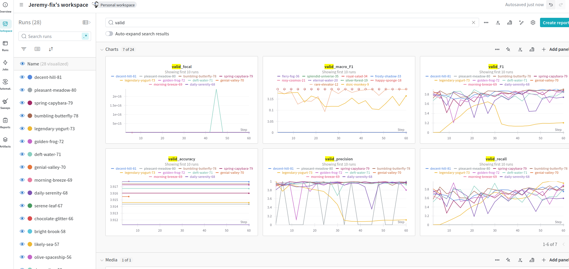
Interfacing with an online dashboard : wandb.ai
As you may expect, deep learning is about tuning your whole pipeline, experimenting with different models and so on and you need to efficiently track all the experiments you will be running.
One part of the answer lies in using dashboards, especially online dashboard are super useful. One such dashboard is wandb.ai. To monitor your experiments with wandb, you just need to add few lines of code.
First, you need to get an account on wandb. This is free and academics have free plans. Once you have an account, you can create a new project, for which you will obtain both a project name and an entity name.
Then you can connect to your wandb calling
import wandb
wandb.init(project=..., entity=....)
and finally, to record your metrics during training, you simply need to call the following function after every epoch :
wandb.log({my_metric_name: my_metric_value})
In our case, we have two dictionnaries train_metrics and test_metrics which contain our metrics, we just need to call wandb.log on them to get your metrics logged :
Running the code without jupyter
Between you and me, a jupyter notebook is great for exploring some concepts but you definitely want to move away from these if you really want to make large scale experiments because running jupyter notebooks is not the most efficient way to perform multiple experiments.
Actually, I adapted a python library I wrote for plankton segmentation so that you are able to evaluate everything from within a notebook.
The library is available on github at https://github.com/jeremyfix/2024_ml4oceans. Feel free to make use of it. You are also provided with a python script submit_slurm.py which allows you to easily run experiments on clusters managed by SLURM (e.g. Jean Zay). Note you will certainly have to adapt the slurm sbatch directives to make it work (e.g. partition name, ...)