Introduction to deep learning based object detection and semantic segmentation
Jeremy Fix, https://jeremyfix.github.io/2024_ml4oceans/
April 23, 2025
Slides made with slidemakerExtracting features with convolutions
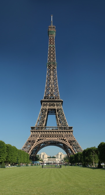
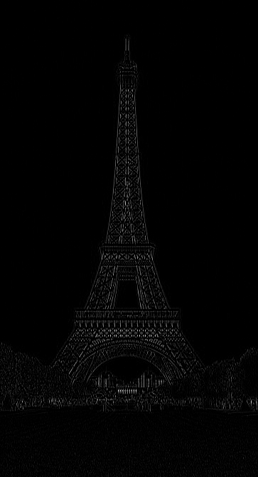
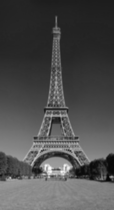
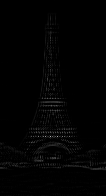
From data that have a spatial structure (locally correlated), features can be extracted with convolutions.
On Images

That also makes sense for temporal series that have a structure in time.
CNN Vocabulary

Convolution :
- size (e.g. \(3 \times 3\), \(5\times 5\))
- padding (e.g. \(1\), \(2\))
- stride (e.g. \(1\))
Pooling (max/average):
- size (e.g. \(2\times 2\))
- padding (e.g. \(0\))
- stride (e.g. \(2\))
We work with 4D tensors for 2D images, 3D tensors for nD temporal series (e.g. multiple simultaneous recordings), 2D tensors for 1D temporal series
In Pytorch, the tensors follow the Batch-Channel-Height-Width (BCHW, channel-first) convention. Other frameworks, like TensorFlow or CNTK, use BHWC (channel-last).
Problem statement
Given :
- images \(x_i\),
- targets \(y_i\) which contains objects bounding boxes and labels
Examples from ImageNet (see here)
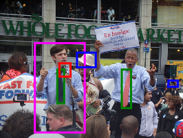
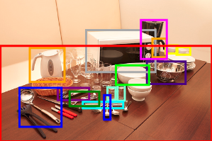
Bounding boxes given, in the datasets (the predictor parametrization may differ), by : \([x, y, w, h]\), \([x_{min},y_{min},x_{max},y_{max}]\), …
Datasets : Coco, ImageNet, Open Images Dataset
Recent survey : (Zou, Chen, Shi, Guo, & Ye, 2023) , (Terven, Córdova-Esparza, & Romero-González, 2023)
Metrics to measure the performances
The metrics should ideally capture :
- the quality of the bounding boxes
- the quality of the label found in the bounding box
Given the “true” bounding boxes:

Quantify the quality of these predictions
A predictor should output labeled bounding boxes with a confidence score. They output a lot.
Your metric should evaluate the fraction of bbox you correctly detect (TP) and the fraction of bbox you incorrectly detect (FP) or incorrectly miss (FN).
The Pascal/COCO mAP metric
For every class individually, every prediction (that has a sufficiently large confidence assigned by your predictor) of every images are considered :
- a true positive (TP) if IoU with ground truth bbox of the same class is higher than a threshold (say \(IOU > 0.3\))
- a false positive (FP) otherwise or if there is a TP for the same ground truth with a higher confidence (“5 detections (TP) of a single object is counted as 1 correct detection and 4 false detections”)
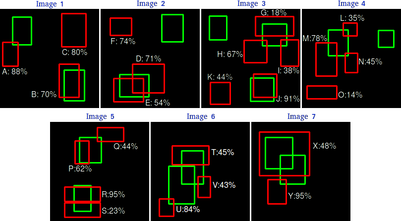
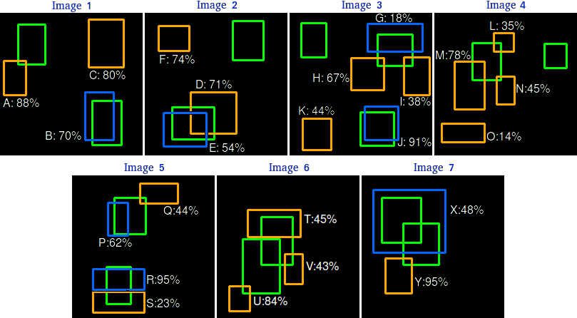
The GT boxes that are not predicted are False Negatives (FN).
Examples from the Object detection metrics repository.
The Pascal/COCO mAP metric
\[ \mbox{precision} = \frac{TP}{TP+FP} \] Which fraction of your detections are actually correct.
\[ \mbox{recall} = \frac{TP}{TP+FN} = \frac{TP}{\#\mbox{gt bbox}} \] Which fraction of labeled objects do you detect (can only increase with decreasing confidence)
If you lower your confidence threshold, your precision can either increase or decrease, your recall can either stall or increase.
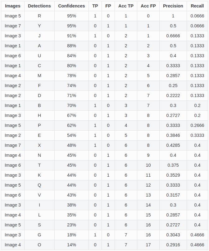
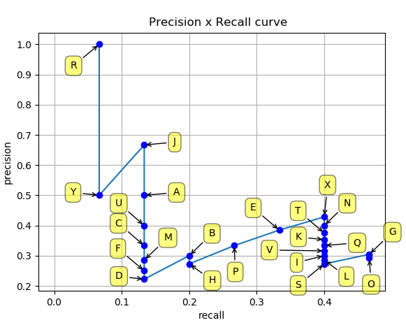
AP is the average precision for different levels of recall. mAP is the average of AP for every classes/categories. Depends on a specific IOU to define TP/FP. Pascal uses mAP@0.5 while COCO averages map@0.5-0.95.
Examples from the Object detection metrics repository.
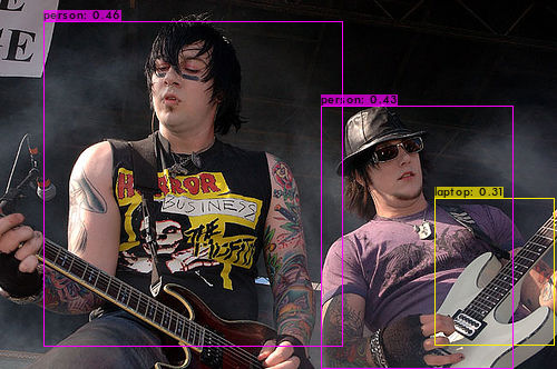
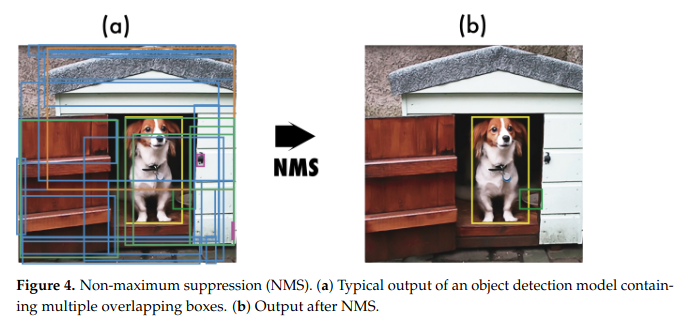
Postprocessing : Non maximum suppression (NMS)
Your predictor will output a lot of bounding boxes. Several might be overlapping.
Non-maximum suppression (NMS) removes lower scoring boxes that overlap (IOU) with other higher scoring boxes.
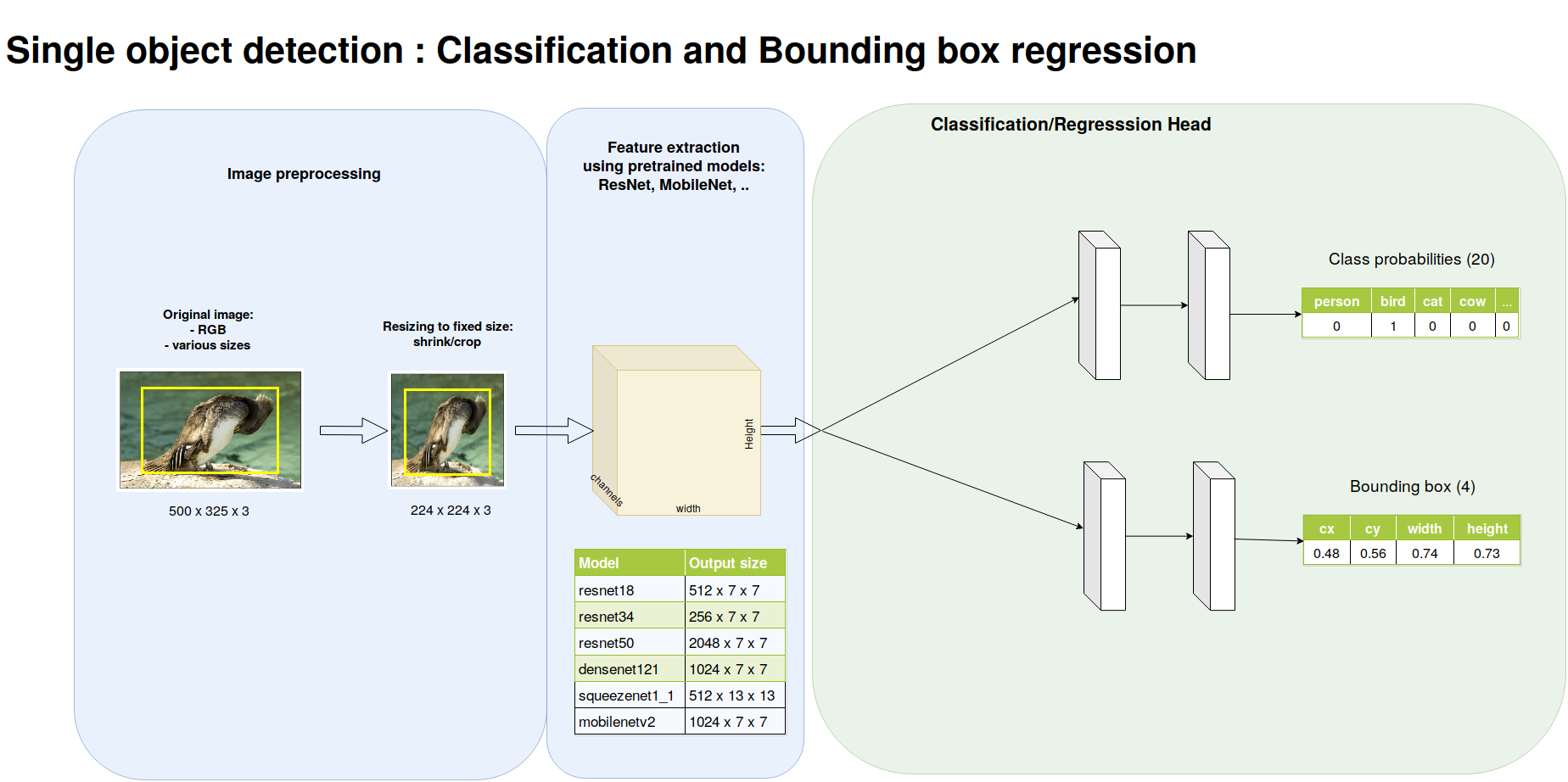
A first step: object localization
Suppose you have a single object to detect, can you localize it into the image ?
The field is moving at a very high pace
As reviewed in [Zhou et al, 2023] :

Region Based Convolutional Neural Network : R-CNN
How can we proceed with multiple objects ? (Ross Girshick, Donahue, Darrell, & Malik, 2014) proposed to :
- use selective search for proposing bounding boxes
- to classify with a SVM from the features extracted by a
pretrained DNN.
- to optimize localization with linear bbox adaptors
Revolution in the object detection community (vs. “traditional” HOG like features).

Drawback :
- external algorithm (not in the computational graph, not trainable)
- one forward pass per bounding box proposal (\(\sim 2K\) or so) \(\rightarrow\) training and test are slow (\(47 s.\) per image with VGG16)
Notes : pretained on ImageNet, finetuned on the considered classes with warped images. Hard negative mining (boosting).
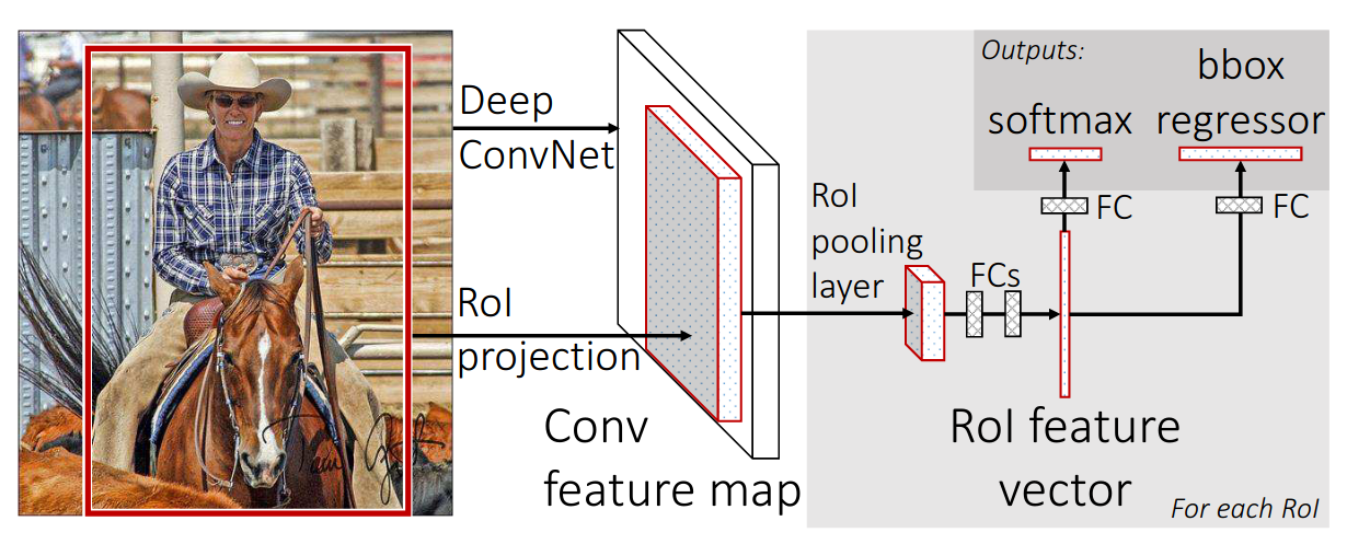
Fast R-CNN
Introduced in (R. Girshick, 2015). Idea:
- just one forward pass
- cropping the convolutional feature maps (e.g. \((1, 512, H/16, W/16)\) conv5 of VGG16)
- max-pool the variable sized crop to a fixed-sized (e.g. \(7 \times 7\)) vector before dense layers: ROI pooling
Drawbacks:
- external algorithm for ROI proposals: not trainable and slow
- ROIs are snapped to the grid (see here) \(\rightarrow\) ROI align
Github repository. CVPR’15 slides
Notes : pretrained VGG16 on ImageNet. Fast training with multiple ROIs per image to build the \(128\) mini batch from \(N=2\) images, using \(64\) proposals : \(25\%\) with IoU>0.5 and \(75\%\) with \(IoU \in [0.1, 0.5[\). Data augmentation : horizontal flip. Per layer learning rate, SGD with momentum, etc..
Multi task loss : \[ L(p, u, t, v) = -\log(p_u) + \lambda \mbox{smooth L1}(t, v) \]
The bbox is parameterized as in (Ross Girshick et al., 2014). Single scale is more efficient than multi-scale.
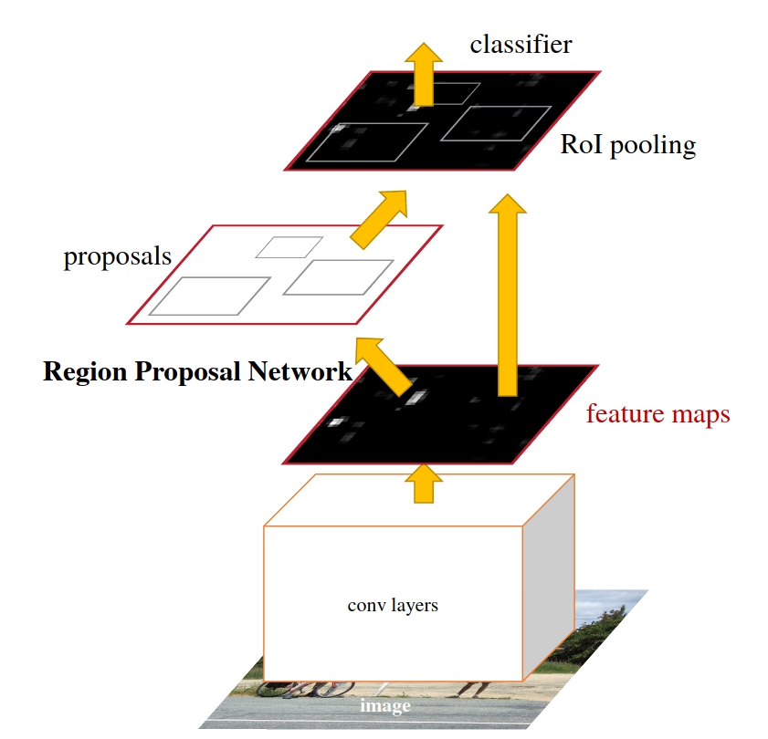
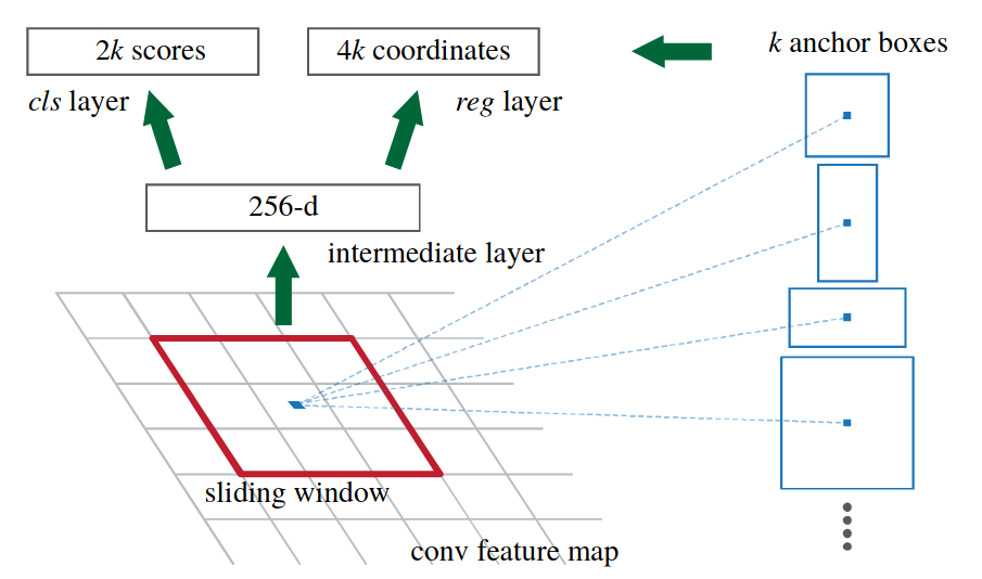
Faster R-CNN : 2-stages trained end-to-end
Introduced in (Ren, He, Girshick, & Sun, 2016). The first end-to-end trainable network. Introducing the Region Proposal Network (RPN). A RPN is a sliding Conv(\(3\times3\)) - Conv(\(1\times1\), k + 4k) network (see here). It also introduces anchor boxes of predefined aspect ratios learned by vector quantization.
Check the paper for a lot of quantitative results. Small objects may not have a lot of features.
Bbox parametrization identical to (Ross Girshick et al., 2014), with smooth L1 loss. Multi-task loss for the RPN. Momentum(0.9), weight decay(0.0005), learning rate (0.001) for 60k minibatches, 0.0001 for 20k.
Multi-step training. Gradient is non-trivial due to the coordinate snapping of the boxes (see ROI align for a more continuous version)
With VGG-16, the conv5 layer is \(H/16,W/16\). For an image \(1000 \times 600\), there are \(60 \times 40 = 2400\) anchor boxes centers.
Multi-scale features with semantic and localization
- In deep classifiers, the top layers are semantically rich but spatially poor,
Feature Pyramid Networks (FPN) (Lin et al., 2017) introduced top-down path to propagate semantics up to the first layers,
Bottom-up path aggregation adds shortcuts to propagate accurate object boundaries to the top layers (Liu, Qi, Qin, Shi, & Jia, 2018)
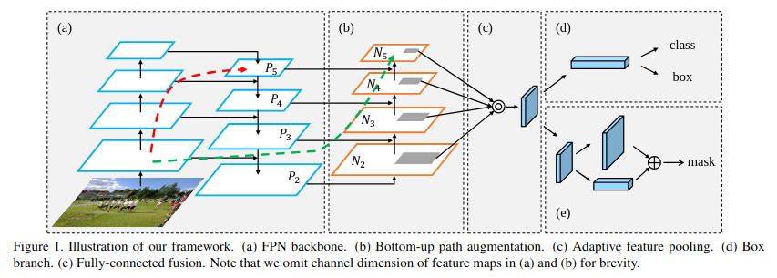
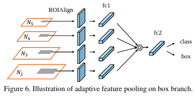
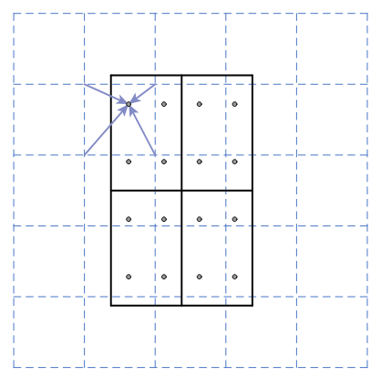
(Liu et al., 2018) also introduced Adaptive Feature Pooling rather than arbitrary assignement of proposals to one level of the pyramid as in (Lin et al., 2017).
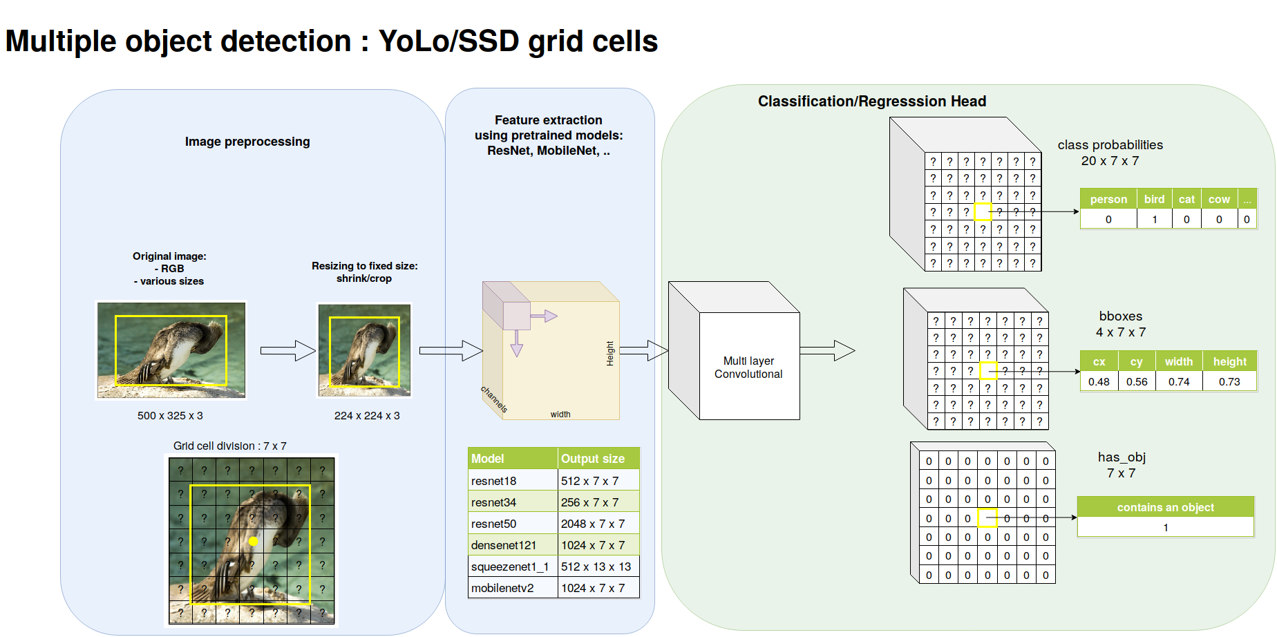
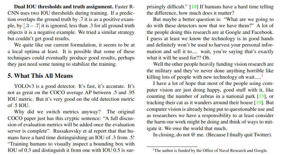
You Only Look Once (Yolo v1,v2,v3)
The first one-stage detector. Introduced in (Redmon, Divvala, Girshick, & Farhadi, 2016). It outputs:
- \(B\) bounding boxes \((x, y, w, h, conf)\) for each cell of a \(S\times S\) grid
- the probabilities over the \(K\) classes
- the output volume is \((5\times B+K)\times(S\times S)\) in YoloV1, then \((5+K)\times B \times (S\times S)\) from v2
Bounding box encoding:
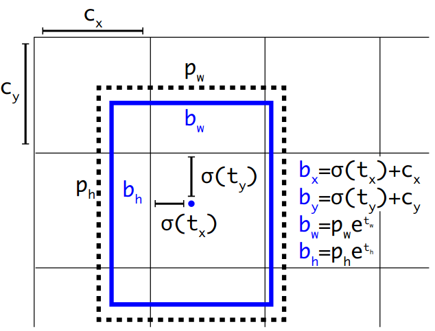
In YoLo v3, the network is Feature Pyramid Network (FPN) like with a downsampling and an upsampling paths, with predictions at 3 stages.
Yolo family
Starting from Yolov4, several authors release some Yolo… version, see (Terven et al., 2023)
- Yolov1 (2016), v2, v3 (2018 )by J. Redmon and al. : principle + anchors + multi-scale (FPN)
Yolov4 (2020), YoloR (2021), Yolov7 (2022) : CSPResNet (cheap DenseNet), bag of freebies (Mosaic, CutMix, Cosine Annealing), bag of specials
YoloX (2021) by Megvii based on Yolo v3 : Anchor free, decoupled heads
Yolov5 (2020), Yolov8 (2023), Yolov11(2024) by Ultralytics
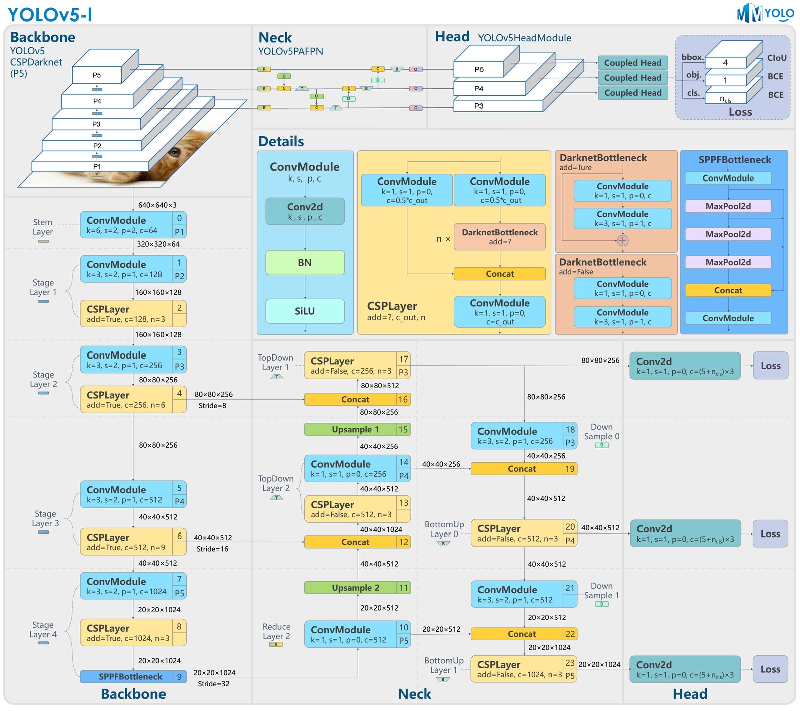
Yolov5 (2020)
- Released in 2020 by Ultralytics
- CSPLayer (cheap DarknetNet from Yolov3 (cheap ResNet))
- Coupled heads, anchor based
- Top-down FPN
- Bottom-up PAN
See also this page
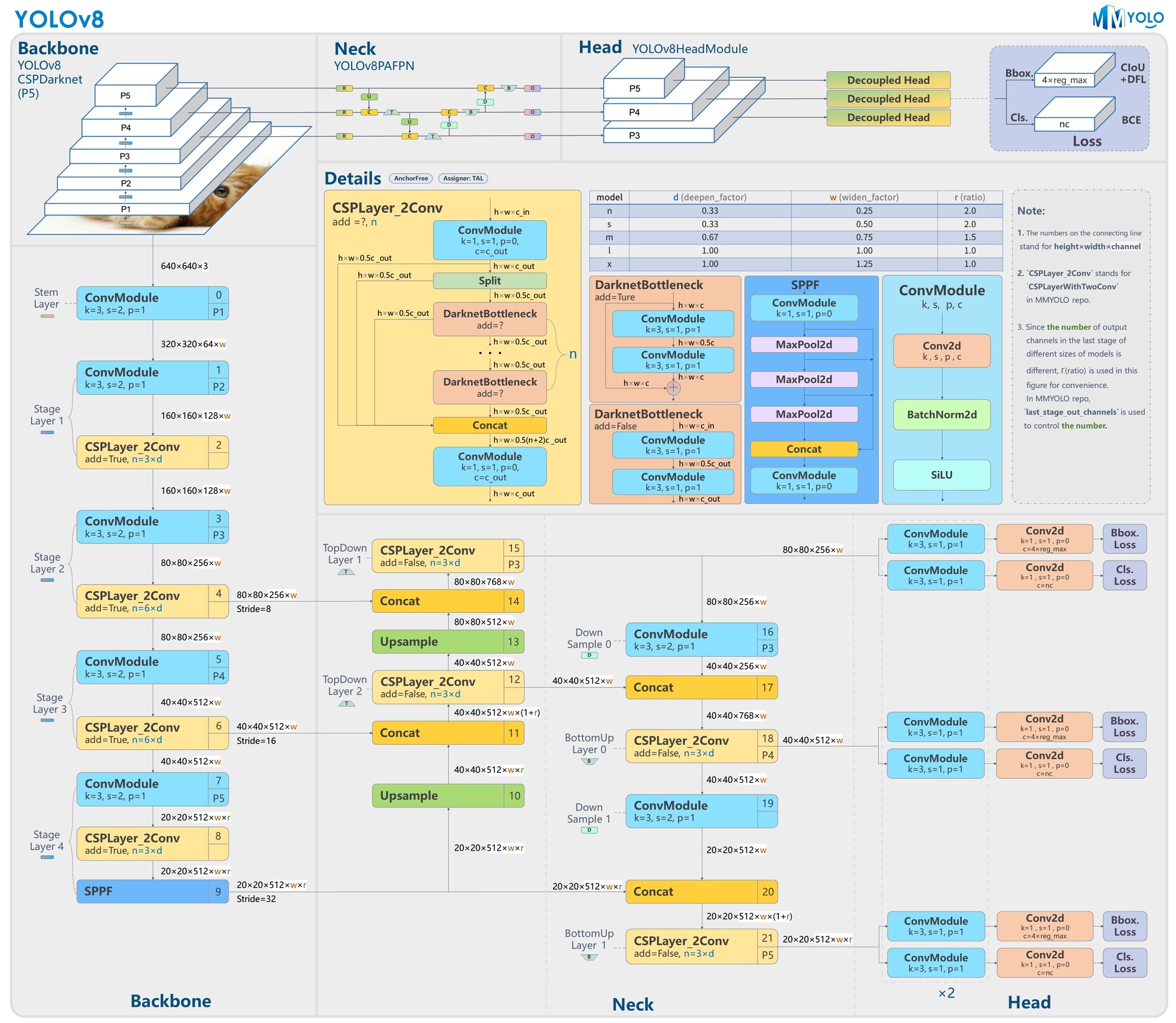
Yolov8 (2023)
- Released early 2023 by Ultralytics
- different scaled versions available (nano … extra-large)
- Updated CSPLayer : C2f module
- Decoupled heads, Anchor free
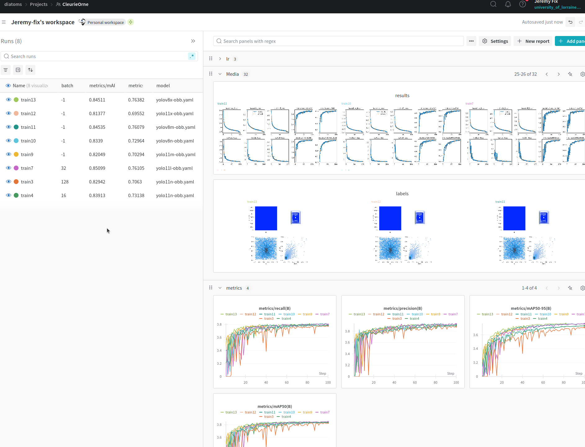
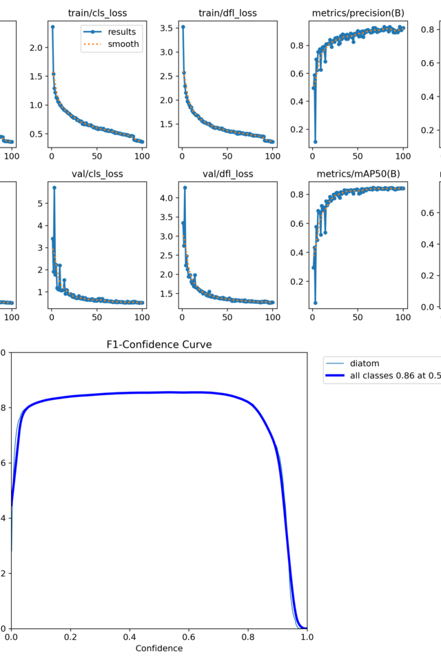
In practice : detecting oriented diatoms
Task: detecting diatoms using oriented bounding boxes (with M. Laviale, C. Pradalier, C. Regan, A. Venkataramanan, C. Galinier)
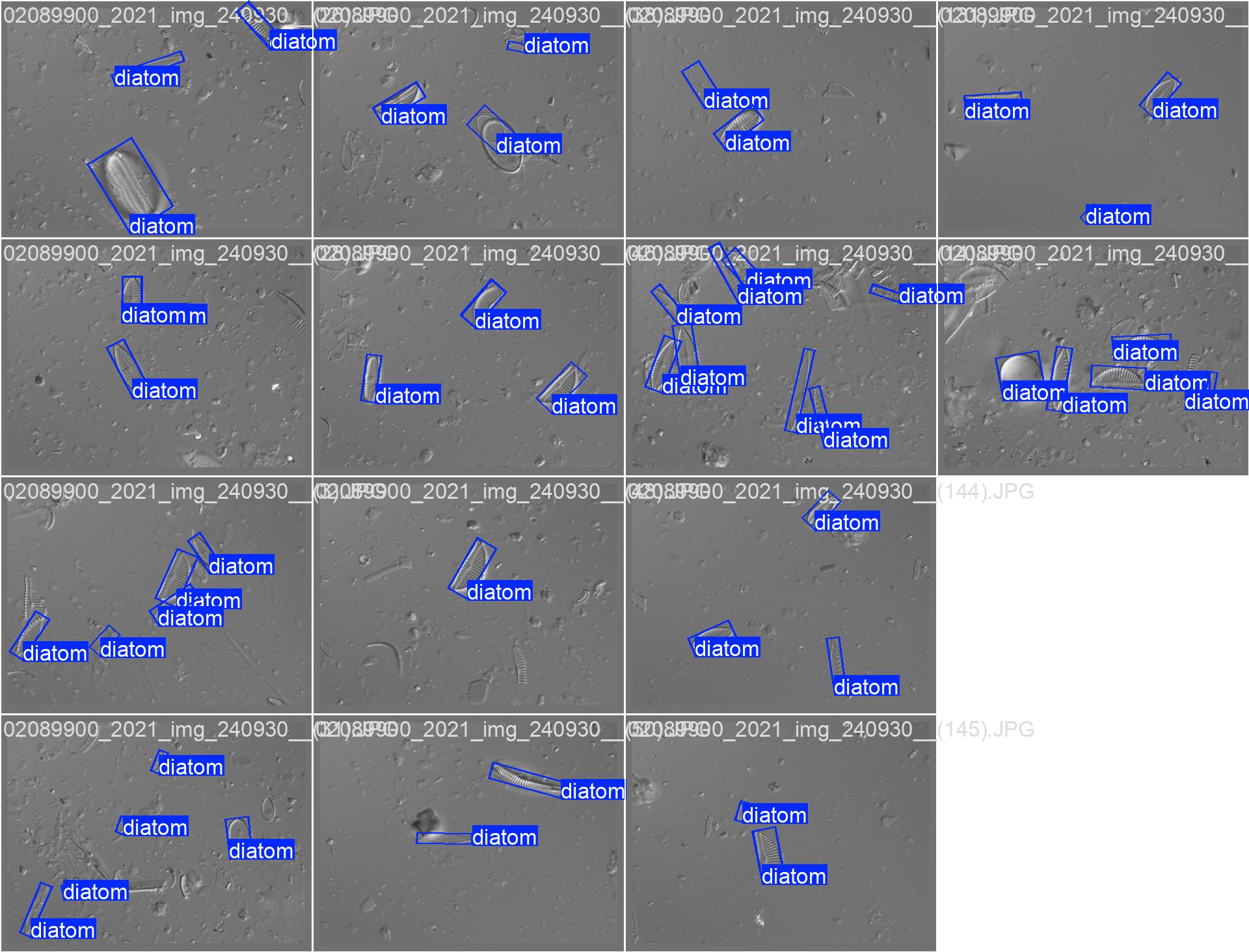
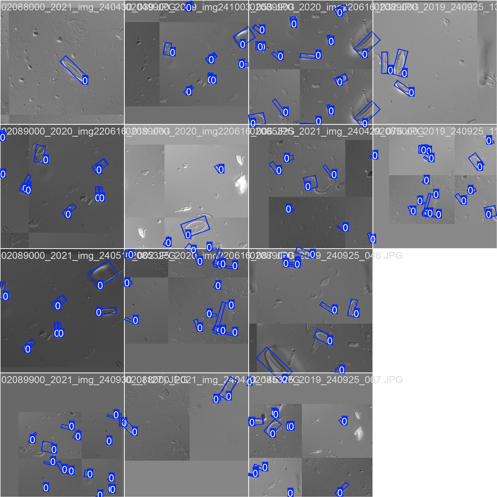
Using ultralytics and their wandb callbacks 😍 ;
Code and instructions on https://github.com/jeremyfix/diatoms_yolo.
Running on IMagine and Teratotheca.
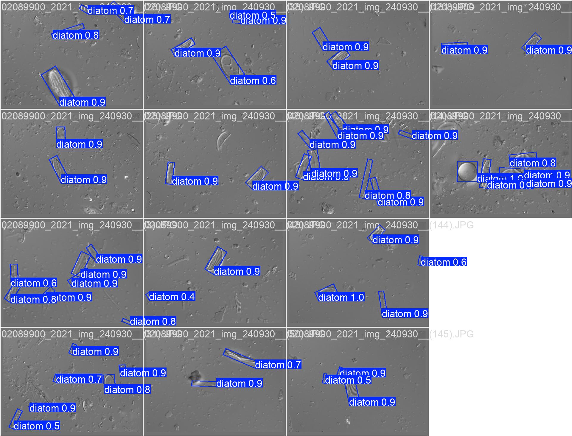
In practice : detecting oriented diatoms (cont. )
Task: detecting diatoms using oriented bounding boxes (with M. Laviale, C. Pradalier, C. Regan, A. Venkataramanan, C. Galinier)
Using ultralytics and their wandb callbacks 😍
Code and instructions on https://github.com/jeremyfix/diatoms_yolo.
Running on IMagine and Teratotheca.
Problem statement
Given an image,
Semantic segmentation : predict the class of every single pixel. We also call dense prediction/dense labelling.
Example image from MS Coco
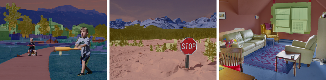
Instance segmentation : classify all the pixels belonging to the same countable objects
Example image from MS Coco
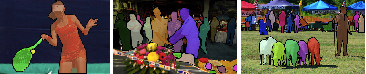
More recently, panoptic segmentation refers to instance segmentation for countable objects (e.g. people, animals, tools) and semantic segmentation for amorphous regions (grass, sky, road).
Metrics : see Coco panotpic evaluation
Some example networks : PSP-Net, U-Net, Dilated Net, ParseNet, DeepLab, Mask RCNN, …
Sliding a classifier
Introduced in (Ciresan, Giusti, Gambardella, & Schmidhuber, 2012).
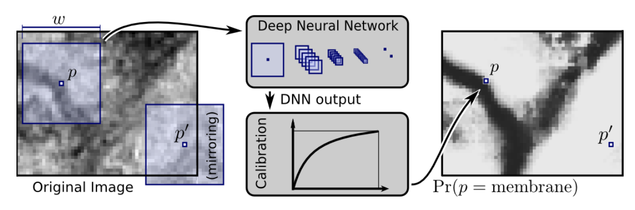
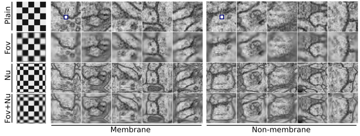
- The predicted segmentation is post-processed with a median filter
- The output probability is calibrated to compensate for different priors on being a membrane / not being a membrane.
Drawbacks:
- one forward pass per patch
- overlapping patches do not share the computations
(on deep neural network calibration, see also (Guo, Pleiss, Sun, & Weinberger, 2017))
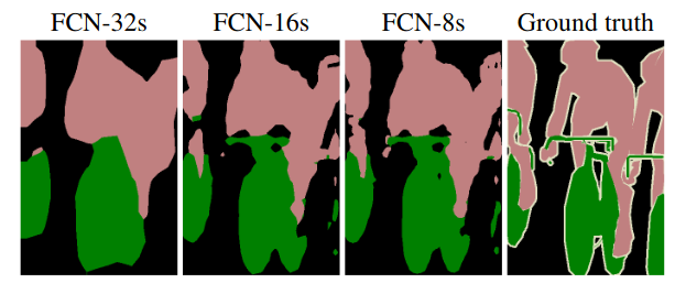
Fully Convolutional Network (FCN)
Introduced in (Long, Shelhamer, & Darrell, 2015). First end-to-end convolutional network for dense labeling with pretrained networks.
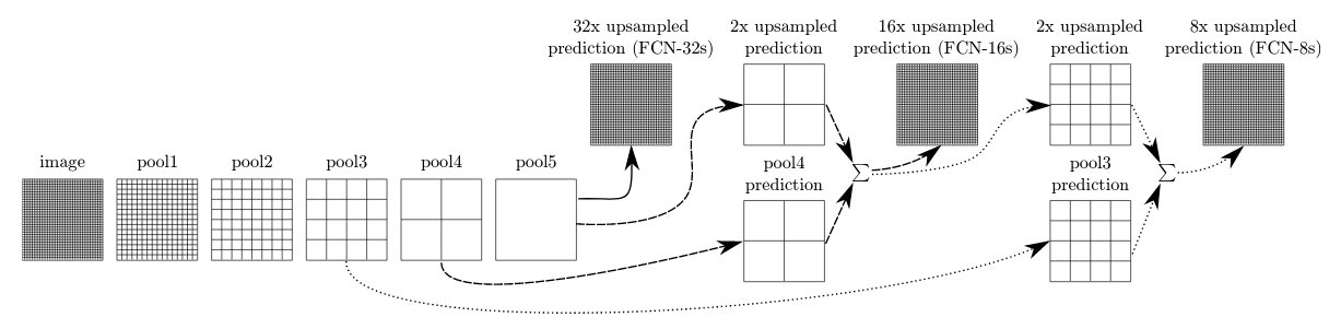
The upsampling can be :
- differentiable hardcoded: e.g. nearest, bilinear, bicubic
- learned as a fractionally strided convolution (deconvolution),
Learned upsampling : fractionally strided convolution
Traditional approaches involves bilinear, bicubic, etc… interpolation.
For upsampling in a learnable way, we can use fractionally strided convolution. That’s one ingredient behind Super-Resolution (Shi, Caballero, Huszár, et al., 2016).

You can initialize the upsampling kernels with a bilinear interpolation kernel. To have some other equivalences, see (Shi, Caballero, Theis, et al., 2016). See ConvTranspose2d.
This can introduce artifacts, check (Odena, Dumoulin, & Olah, 2016). Some prefers a billinear upsampling, followed by convolutions.
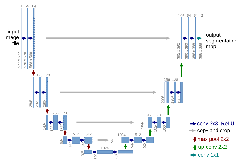
Encoder/Decoder architectures
Several models along the same architectures : SegNet (sum), U-Net (concat). Encoder-Decoder architecture introduced in (Ronneberger, Fischer, & Brox, 2015)
There is :
- a contraction path from the image “down” to high level features at a coarse spatial resolution
- an expansion upsampling path which integrates low level features for pixel wise labelling
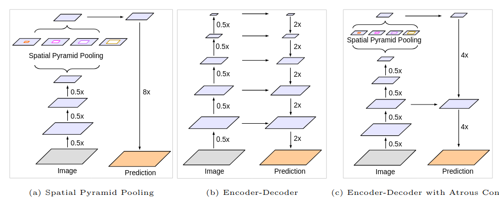
DeepLab
To gather contextual information by enlarging the receptive fields, DeepLab employs “a-trou” convolutions (dilated) rather than max pooling. DeepLabV1 (Chen, 2014), DeepLabV2 (Chen, Papandreou, Kokkinos, Murphy, & Yuille, 2017), DeepLabV3 (Chen, Papandreou, Schroff, & Adam, 2017), DeepLabV3+ (Chen, Zhu, Papandreou, Schroff, & Adam, 2018).
- Max-pooling in classification backbones induces invariance to translation \(\rightarrow\) a-trou convolutions
- How to deal with objects at multiple scales ? \(\rightarrow\) Atrous Spatial Pyramid Pooling (ASPP)
- In DeepLabV3+, combines with some decoding upsampling layers
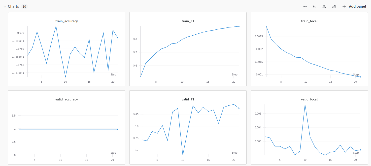
In practice
Task Segment non-living stuff vs living organisms in ZooScan images.
- Large images \(\approx 15000 \times 23000\) containing objects belonging to \(89\) categories. Non living (label < 8) or living.
- Using either :
- a UNet with a pretrained backbone + random decoder (lab)
- a DeepLabv3+ pretrained on ImageNet
- Trained on \(512 \times 512\) overlapping patches, focal loss, F1 score for early stopping
- 76K for training, 19K for validation
- One epoch in 10 minutes on RTX 3090
- Flip, Rotate, MaskDropout, Blur
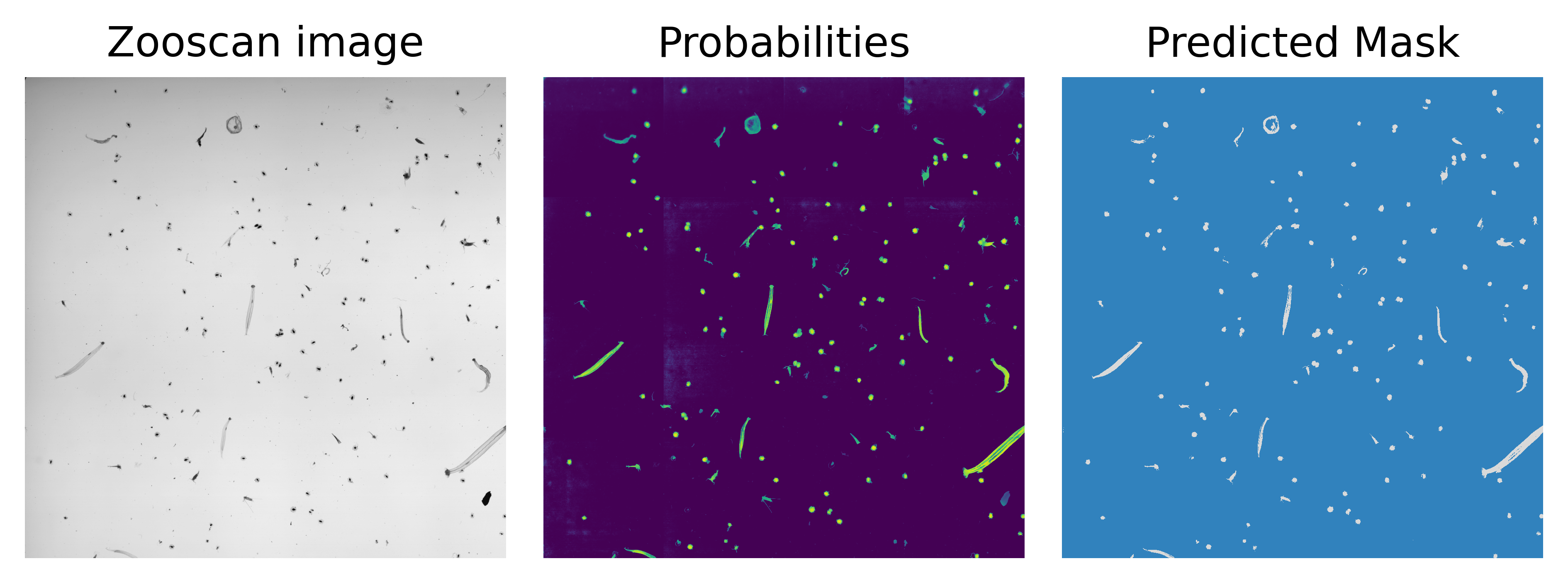
In practice
Task Segment non-living stuff vs living organisms in ZooScan images.
Inference on a new sample with tiled inference. We could have used averaged inference with overlapping tiles.
Mask produced with threshold@0.5 which may be suboptimal.
Mask-RCNN
Introduced in (He, Gkioxari, Dollár, & Girshick, 2018) as an extension of Faster RCNN. It outputs a binary mask in addition the class labels + bbox regressions.
It addresses instance segmentation by predicting a mask for individualised object proposals.
Proposed to use ROI-Align (with bilinear interpolation) rather than ROI-Pool.
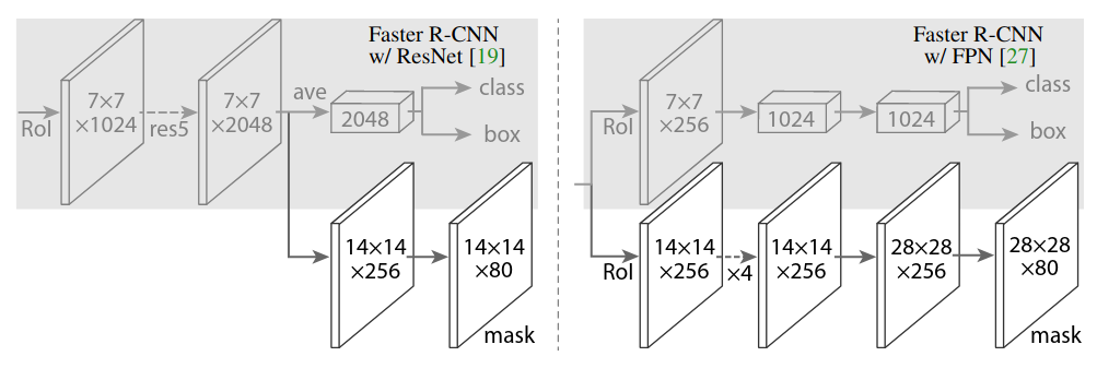
There is no competition between the classes in the masks. Different objects may use different kernels to compute their masks.
Can be extended to keypoint detection, outputting a \(K\) depth mask for predicting the \(K\) joints.
Transformers
Introduced in (Vaswani et al., 2017), from NLP to Vision by ViT (Dosovitskiy et al., 2021).
Recent propositions for :
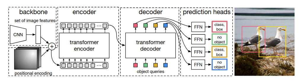
- Object detection : (Carion et al., 2020) proposed a transformer based object detector. The decoder outputs a predefined large number \(N\) of labeled bounding boxes.
In practice, huggingface transformers implements DETR. Look at the paper, it is just few lines of pytorch.
- Semantic segmentation : FAIR introduced self-supervized Segment Anything Model (Kirillov et al., 2023).In practice, have a look to https://github.com/facebookresearch/segment-anything.
- General purpose self-supervised foundation model DinoV2 (Oquab et al., 2023), (Darcet, Oquab, Mairal, & Bojanowski, 2023). In practice, huggingface trasnformers implements DINOv2, code by FAIR