Python pour les scientifiques

Une rapide introduction

Jeremy Fix

CentraleSupélec

Python: classes, threads, UI, packaging

Un problème pour se motiver

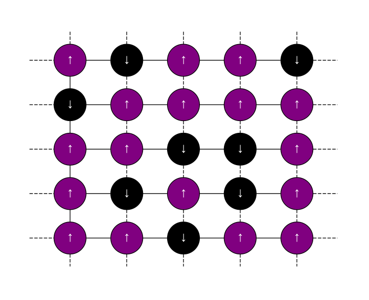
Problème Simuler un système d’Ising (Sethna (2006), Hayes (2000)). Moment magnétique des atomes arrangés sur une grille régulière \(\sigma_i \{-1, 1\}\). Pour une grille finie, il existe un nombre fini de configurations mais avec des dynamiques intriguantes.

La probabilité d’occuper un état du système \(\sigma\) est \(P(\sigma) = \frac{1}{Z}\exp(-\beta E(\sigma))\), avec

\[ E(\sigma) = -\sum_{i < j} J_{i,j} \sigma_i \sigma_j \]

• transition déterministe si l’énergie globale diminue, \(\Delta E < 0\),
• transition stochastique si l’énergie augmente \(\Delta E > 0\), avec probabilité \(\exp(-\beta \Delta E) \in [0, 1]\)

Système de Ising

Il existe des transitions de phase, en particulier pour \(\beta \approx 2.269\).

Voir la description complète du système sur https://tutos.metz.centralesupelec.fr/TPs/Intro-Python/index.html#an-example-project-simulating-the-ising-model

Les classes

Concept fondamental de programmation orientée objet (OOP).

• Un objet = des attributs modifiables par des méthodes qui forment un tout cohérent. On parle aussi de classe,
• Une réalisation d’un objet est appelée une instance,
• peut être organisé de manière hiérarchique,
• peut redéfinir/spécifier des opérations

On peut construire une instance d’un objet :

class MaClasse:
  
  # Constructeur
  def __init__(self, ...):
    pass

On dispose également de beaucoup de méthodes spéciales : __lt__, __add__, __str__, …

On peut construire une hiérarchie de classes, on doit alors appeler le constructeur de la classe mère.

Illustrations de la programmation orientée objet

Problème Écrire un évaluateur d’expressions mathématiques.

from abc import ABC, abstractmethod

class Expression(ABC):
    @abstractmethod
    def __str__(self):
        pass

    @abstractmethod
    def __call__(self, env):
        pass

class Variable(Expression):
    def __init__(self, name):
        self.name = name

    def __call__(self, env):
        return env[self.name]

    def __str__(self):
        return self.name

class BinaryOp(Expression):
    def __init__(self, fun, left, right):
        self.fun = fun
        self.left, self.right = left, right

    def __call__(self, env):
        return self.fun(self.left(env), self.right(env))

class Add(BinaryOp):
    def __init__(self, left, right):
        super().__init__(lambda x, y: x+y, left, right)

    def __str__(self):
        return f"({self.left} + {self.right})"

class Multiply(BinaryOp):
    def __init__(self, left, right):
        super().__init__(lambda x, y: x*y, left, right)

    def __str__(self):
        return f"({self.left} * {self.right})"

Exemple

# Exemple usage
# expr = parse("3 * x + 2")

expr = Add(Multiply(Constant(3), Variable('x')), Constant(2))

print(expr)  # (3 * x + 2)
print(expr.evaluate({'x': 5}))  # 17

Les classes

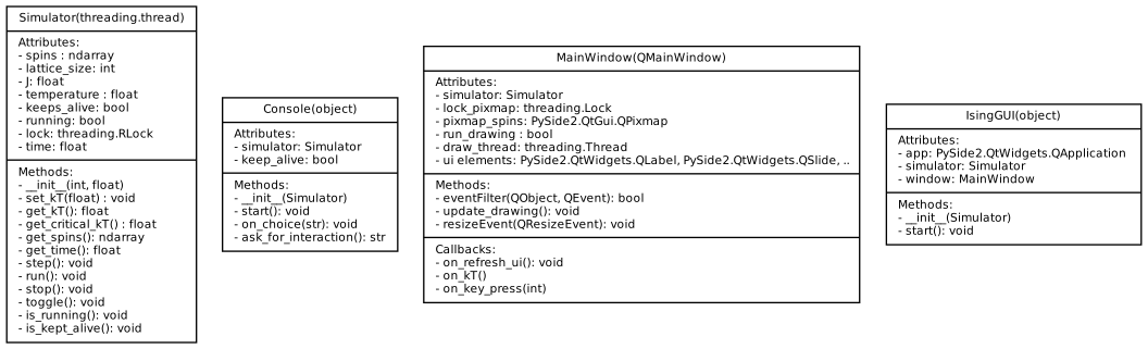
On décompose le projet en \(3\) classes :

• un simulateur qui s’occupe de la physique
• une interface en ligne de commande Console
• une interface graphique IsingGUI

Diagramme de classes

Les threads ?

Un programme peut déclencher plusieurs fils d’exécutions, les threads. Ici :

• un thread pour le simulateur
• un thread pour l’interaction avec l’utilisateur (le principal)

Cela permet à la simulation de continuer à tourner même si l’utilisateur n’interagit pas.

class Console(object):
    def __init__(self, simu):
        self.simulator = simu

    def ask_for_interaction(self):
      ...

    def on_choice(self, choice):
      ...

    def start(self):
        """
        The main loop
        """
        while self.keep_alive:
            choice = self.ask_for_interaction()
            self.on_choice(choice)

import threading
class Simulator(threading.Thread):

    def __init__(self, lattice_size, kT):
        threading.Thread.__init__(self)
        self.lock = threading.RLock()
        self.spins = np.random.random((lattice_size, lattice_size)) > 0.5

    def run(self):
        while self.is_kept_alive():
            if self.running:
                self.step()

    def stop(self):
        with self.lock:
            self.keeps_alive = False

    def get_spins(self):
        with self.lock:
            return self.spins.copy()

Au lieu des threads, on aurait pu utiliser du multiprocessing.

Installation et exécution

Installation (grâce au setup.py)

uv venv /tmp/venv
source /tmp/venv/bin/activate
uv pip install -e ising_package

Exécution

python -m ising.console
python -m ising.qtgui

Packaging du projet

Le projet est packagé avec setuptools.

La python packaging authority (pypa) maintient un tutorial sur le packaging, voir https://setuptools.pypa.io/en/latest/userguide/quickstart.html

Le packaging peut se faire avec un setup.py :

import setuptools

with open("README.md", "r") as fh:
    long_description = fh.read()

setuptools.setup(
    name="Ising",
    version="1.0",
    author="CentraleSupelec",
    author_email="Jeremy.Fixcentralesupelec.fr",
    description='A simulator of the Ising model with '
                'the Metropolis algorithm',
    long_description=long_description,
    long_description_content_type="text/markdown",
    url='http://tutos.metz.centralesupelec.fr/Intro_Python',
    packages=setuptools.find_packages(),
    classifiers=[
        "Programming Language :: Python :: 3",
        "License :: OSI Approved :: MIT License",
        "Operating System :: OS Independent",
    ],
    python_requires='>=3.6',
    install_requires=['numpy', 'scipy', 'PyQt5', 'matplotlib', 'opencv-python-headless']
)

Mais pourrait aussi utiliser pyproject.toml.

Et vous pourriez déposer votre librairie sur pypi, ou conda.

Calcul scientifique avec Numpy

Introduction

Numpy : Numerical Python

• Librairie C++ avec un wrapper python,
• qui offre des tableaux multi-dimensionnels et des opérations optimisées

NumPy is the fundamental package for scientific computing in Python. It is a Python library that provides a multidimensional array object, various derived objects (such as masked arrays and matrices), and an assortment of routines for fast operations on arrays, including mathematical, logical, shape manipulation, sorting, selecting, I/O, discrete Fourier transforms, basic linear algebra, basic statistical operations, random simulation and much more.

• Documentation : https://numpy.org/doc/stable/,
• Tutoriels : https://lectures.scientific-python.org/intro/numpy/index.html et sur les Quickstart sur la page de documentation,
• Le “Try it in your browser!”, voir par exemple le bas de https://numpy.org/doc/2.3/reference/generated/numpy.linalg.inv.html
• Code source : https://github.com/numpy/numpy

import numpy as np

Création de tableaux

Plusieurs approches pour créer un tableau Numpy :

• à partir d’une liste (éventuellement de listes de listes de ..)
• à partir de fonctions dédiées : np.zeros, np.ones, np.arange, np.linspace, np.random.rand, etc.
• à partir de fichiers : np.loadtxt, np.genfromtxt, np.load, etc.

# Tableau 1D de taille (5, )
np.array([1, 2, 3, 4, 5])

# Tableau 2D de taille (2, 3)
np.array([[1, 2, 3], [4, 5, 6]])

# Tableau 2D de taille (3, 4) rempli de zéros
np.zeros((3, 4))

# Tableau 6D de taille (2, 3, 4, 5, 6, 7) rempli de uns
np.ones((2, 3, 4, 5, 6, 7))

# Tableau 1D de 0 à 10 par pas de 2
np.arange(0, 10, 2)

# Tableau 1D de taille (5, ) avec des valeurs entre 0 et 1
np.linspace(0, 1, 5)

# Tableau 2D de taille (3,3) avec des valeurs aléatoires entre 0 et 1
np.random.rand(3, 3)

Propriétés des tableaux

Les tableaux ont :

• une forme (shape) : nombre de dimensions et taille dans chaque dimension,
• un type (dtype) : type des éléments du tableau,
• un nombre d’éléments (size) : nombre total d’éléments dans le tableau,
• un nombre de dimensions (ndim) : nombre de dimensions du tableau.

a = np.array([[1, 2, 3], [4, 5, 6]])
print(a)

print("Shape:", a.shape)      # (2, 3)
print("Dtype:", a.dtype)      # int64 (ou int32 selon la plateforme)
print("Size:", a.size)        # 6
print("Ndim:", a.ndim)        # 2

Accès aux éléments

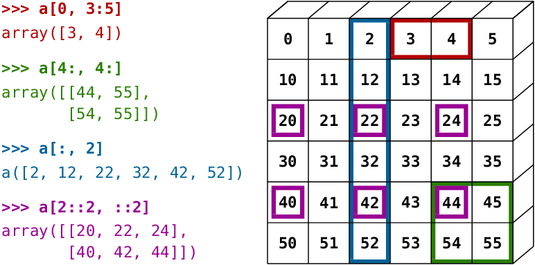
On accède aux éléments :

• par index,
• par slicing, en utilisant la syntaxe python start:stop:step,
• par masquage booléen

Illustration de slicing de https://lectures.scientific-python.org/intro/numpy/array_object.html

Pour l’efficacité en mémoire et temps:

• le slicing crée une vue sur le tableau original, pas une copie.
• Mais, le fancy indexing crée une copie, pas une vue.

On peut le vérifier avec l’attribut base

a = np.array([[1, 2, 3], [4, 5, 6]])

# Accès par index
# Premier élément de la première ligne
a[0, 0]  # 1

# Accès par slicing
# Deuxième ligne
# Equivalent à a[1]
a[1, :]  # [4 5 6]

# Première colonne
a[:, 0]  # [1 4]

# Toutes les lignes, colonnes d'indice pair
a[:, ::2] #
a[:, ::2] = 0 # Modifie a

# Masquage booléen : fancy indexing
mask = a > 3 # np.array de dtype bool
b = a[mask]  # [4 5 6]
b[0] = 10    # Ne Modifie pas a

Accès aux éléments (suite)

Ne jamais faire

a = np.array([[1, 2, 3], [4, 5, 6]])

for i in range(a.shape[0]):
  for j in range(a.shape[1]):
    a[i, j] = 0

mais utiliser l’ellipsis :

a = np.array([[1, 2, 3], [4, 5, 6]])

a[...] = 0

Manipulations sur la forme des tableaux

On peut modifier la forme d’un tableau par :

• np.reshape : retourne une vue du tableau avec une nouvelle forme,
• np.flatten ou np.ravel : retourne une copie ou une vue du tableau aplati (1D),
• np.transpose : retourne une vue du tableau transposé,
• np.pad : ajoute une bordure autour du tableau.
• np.expand_dims, x = x[np.newaxis, :] : ajoute une nouvelle dimension.

On peut combiner/diviser plusieurs tableaux par :

• np.concatenate : concatène plusieurs tableaux le long d’un axe,
• np.stack : empile plusieurs tableaux le long d’un nouvel axe,
• np.hstack et np.vstack : concatène horizontalement ou verticalement plusieurs tableaux.
• np.split, np.hsplit, np.vsplit : divise un tableau en plusieurs sous-tableaux.

On peut permuter les éléments d’un tableau par :

• np.transpose, np.swapaxes
• np.roll

Opérations arithmétiques sur les tableaux

Les opérations arithmétiques sont appliquées élément par élément +, ‘/’, -, *. Il existe également les opérations logiques.

a = np.array([[1, 2, 3], [4, 5, 6]])
b = np.array([[10, 20, 30], [40, 50, 60]])

# Addition  
c = a + b  # [[11 22 33] [44 55 66]]

# Soustraction
d = b - a  # [[9 18 27] [36 45 54]]

# Multiplication terme à terme
e = a * b  # [[10 40 90] [160 250 360]]

# Division terme à terme
f = b / a  # [[10. 10. 10.] [10. 10. 10.]]

Attention : * est le produit terme à terme, pas le produit matriciel. Le produit matriciel est obtenu par np.matmul ou simplement @

Illustration : Système de GrayScott

Problème

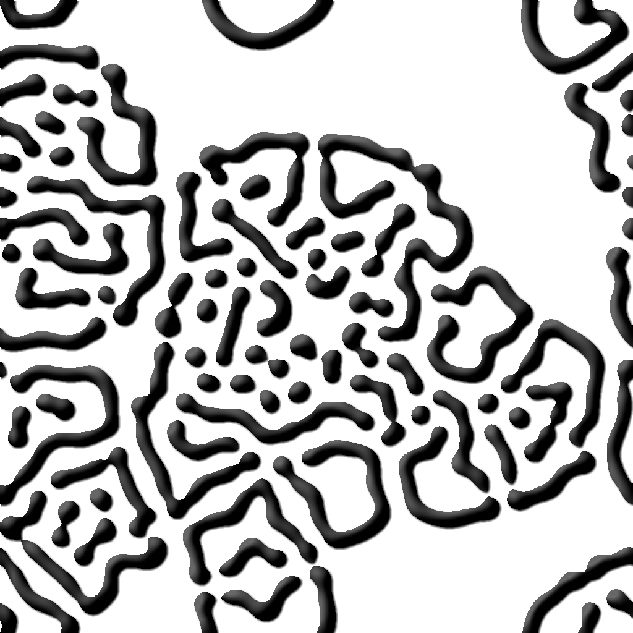
Problème Simuler le système de réaction-diffusion de GrayScott dont l’évolution des champs spatialisés \(u(x,t)\), \(v(x,t)\), \(x\in \mathbb{R}^2\) est régie par :

\[ \begin{eqnarray*} \frac{\partial u}{dt}(x,t) &=& D_u \nabla^2 u(x,t) - u(x,t) v^2(x,t) \\ & &+ F(1-u(x,t))\\ \frac{\partial v}{dt}(x,t) &=& D_u \nabla^2 v(x,t) + u(x,t) v^2(x,t) \\ && - (F+k) v(x,t) \end{eqnarray*} \]

def step(ut_1, vt_1, Du, Dv, F, k):
  uvv = ut_1 * vt_1**2
  lu = laplacian(ut_1)
  lv = laplacian(vt_1)
  ut[...] = ut_1 + dt * (Du * lu - uvv + F*(1-ut_1))
  vt[...] = vt_1 + dt * (Dv * lv + uvv - (F + k) * vt_1)

def laplacian(src):
  """
  u is a 2D nd array
  """
  padded_src = np.pad(src, pad_width=1, mode="constant")  # zero padding src
  laplacian = (
      0
      + padded_src[0:-2, 1:-1]
      + 0
      + padded_src[1:-1, 0:-2]
      - 4 * padded_src[1:-1, 1:-1]
      + padded_src[1:-1, 2:]
      + 0
      + padded_src[2:, 1:-1]
      + 0
  )

  return laplacian[1:-1, 1:-1]

avec \(\nabla^2\) le laplacien discret :

\[ \nabla^2 u(x,y) = \frac{u(x-\delta, y) + u(x+\delta, y) + u(x, y-\delta) + u(x, y+\delta) - 4 u(x,y)}{\delta^2} \]

Illustration - Système de Grayscott

$ uv venv /tmp/venv
$ source /tmp/venv/bin/activate
$ uv pip install numpy scipy opencv-python
$ python cv2_grayscott 4

Grayscott simulation

Calcul avec numpy: Broadcasting

Fonctions Mathématiques

Les fonctions Mathématiques s’appliquent sur tout les éléments, e.g. np.exp, np.sin, np.log, etc mais également les puissances.

e.g. Calcul d’une gaussienne centrée en \(x=2\) avec écart-type \(\sigma=0.5\)

x = np.linspace(0, 4, 100)
sigma = 0.5
gauss = (1/(sigma * np.sqrt(2 * np.pi))) * np.exp(-0.5 * ((x - 2) / sigma) ** 2)

On peut également calculer (selon un axis=..):

• la somme : np.sum,
• le plus petit/grand : np.min, np.max, np.argmin, np.argmax,
• la moyenne : np.mean \(\frac{1}{N} \sum_i X[..., i, ...]\), l’écart type np.std \(\sqrt{\frac{1}{N} \sum_i (X[..., i, ...] - \mu_i)^2}\)
• la covariance : np.cov \(\sum_i (x_i - \mu)^T (x_i - \mu)\)
• …

Broadcasting

Le broadcasting est un mécanisme qui permet d’effectuer des opérations entre des tableaux de formes différentes.

Numpy “étend” automatiquement les dimensions des tableaux pour qu’ils soient compatibles pour l’opération.

De la documentation sur le broadcasting

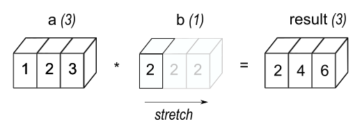
La règle : des opérations sur deux tableaux sont applicables si les dimensions sont compatibles.

Les dimensions sont compatibles si, 1) les tableaux ont le même nombre de dimensions, 2) partant de la droite (des dimensions)

• les dimensions sont égales
• ou sont différentes mais l’une d’elle est égale à \(1\) \(\rightarrow\) Broadcast

Sinon vous obtiendrez l’exception ValueError: operands could not be broadcast together

Broadcasting - example

Par exemple, on souhaite calculer la valeur d’une fonction gaussienne \(f(x)\) centrée en \(\mu\in\mathbb{R}^2\), sur une grille régulière centrée sur \(\mu\) :

\[ \forall x \in \mathbb{R}^2, f(x) = \frac{1}{\sigma \sqrt{2\pi}} \exp(\frac{- \|x - \mu\|_2^2}{2\sigma^2}) \]

if __name__ == '__main__':
    mu = np.array([1, 2])
    sigma = 0.3
    step = 0.1
    Nsteps = 10
    X = gaussian(mu, sigma, step, Nsteps)

def gaussian(mu: np.ndarray, sigma: float, step: float, Nsteps: int) -> np.ndarray:
    # Generate the regular grid
    # (-N, -(N-1), ..., -1, 0, 1, ..., N-1, N) * step
    intsteps = (np.arange(Nsteps) + 1)
    deltasteps = np.concatenate([-intsteps[::-1], [0], intsteps]) * step

    # Generate the steps centered on mu
    # mu is (2, ), we use broadcasting on mu and deltasteps to generate
    # mu (2, 1) + deltasteps(1, M) => mu + deltasteps is (2, M)
    mu_delta = mu[:, np.newaxis] + deltasteps[np.newaxis, :]

    # Generate the meshgrid with this values
    # X and Y are of shape (2*Nsteps + 1, 2*Nsteps + 1)
    X, Y = np.meshgrid(mu_delta[0], mu_delta[1])

    # Concatenate the X, Y matrices
    # xy is  (( (2*Nsteps + 1) * (2*NSteps + 1), 2)
    xy = np.concatenate((X.ravel()[:,np.newaxis], Y.ravel()[:, np.newaxis]), axis=1)

    # Compute tha gausian values
    # To compute the distance between the grid points is computed between xy and mu
    # To broadcast, we do :   xy (M, 2) - mu(1, 2)
    dist = ((xy - mu[np.newaxis, :])**2).sum(axis=1)
    values = 1.0 / (2.0 * sigma * np.sqrt(2.0 * np.pi)) * np.exp(- dist / (2.0 * sigma**2))
    
    # Values is of shape (( (2*Nsteps + 1) * (2*NSteps + 1), ) that we reshape as 
    # (2*Nsteps + 1, 2*Nsteps + 1)
    values = values.reshape((2*Nsteps + 1, 2*Nsteps + 1))

    return values

Calcul avec Numpy: algèbre linéaire

Algèbre linéaire

Numpy supporte bien évidemment toutes les routines utiles en algèbre linéaire, dans le sous-package np.linalg:

• produit matriciel , matrice-vector : np.dot
• calcul de la trace np.linalg.trace,
• calcul de l’inverse : np.linalg.inv, du déterminant np.linalg.det
• calcul des normes : np.norm - norme \(p\) pour un vecteur \((\sum_i x_i^p)^{1/p}\), Frobenius pour une matrice,
• diagonalisation, valeurs propres, vecteurs propres : np.linalg.eig
• décompositions de Cholesky np.linalg.cholesky \(X = L L^T\) (L triangulaire inférieure), SVD np.linalg.svd \(X = U S V^T\)

Algèbre linéaire - illustrations

Moindres carrés régularisés Soit \(n, m \in \mathbb{N}\), \(A\in \mathbb{R}^{n,m}\), \(b\in \mathbb{R}^{n}\), trouver \(x \in \mathbb{R}^m\) qui minimise :

\[ argmin_x J(x) = \|A x - b\|_2^2 = \sum_{i=0}^{n-1} (\sum_{j=0}^{m-1} a_{i,j}x_j - b_i)^2 \]

En fonction du range de \(A\), il peut exister une infinité de solution. Si \(A\) est singulière, une solution est obtenue en résolvant le problème des moindres carrés régularisés \(argmin_x J(x) + \lambda \|x\|_2^2\) , \(\lambda \in \mathbb{R}^+\) :

\[ x = (A^T A + \lambda \mathbf{I})^{-1} A^T b \]

Avec numpy :

import numpy as np

def rls(A: np.ndarray, b: np.ndarray, lbd: float) -> np.ndarray:
    n, m = A.shape
    inv = np.linalg.inv(A.T@A + lbd * np.eye(m))
    x = np.dot(inv@A.T, b)
    return x

if __name__ == '__main__':
    n, m = 3, 4
    A, b = np.random.random((n, m)), np.random.random((n,))
    lbd = 0.001

    x = rls(A, b, lbd)
    print(x)

Algèbre linéaire - PCA

Analyse en composantes principales Soit \(N\) vecteurs \(x_i \in \mathbb{R}^d\), trouver le vecteur \(w_0 \in \mathbb{R}^d\) et \(r\) vecteurs de projections \(w_j\) qui minimisent l’erreur de reconstruction :

\[ \begin{align} \min_{\{w_0, w_1, ..w_r\} \in \mathbb{R}^d} \sum_{i=0}^{N-1} \left|x_i - (w_0 + \sum_{j=1}^r (w_j^T (x_i-w_0))w_j )\right|_2^2 \end{align} \]

sujet à la contrainte \(\forall i, j \geq 1, w_i^T w_j = \delta_{i,j}\).

PCA

Algèbre linéaire - PCA

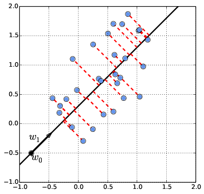
Algorithme:

1. Centrer vos données \(\widetilde{x}_i = x_i - \bar{x}\)
   
2. Construire la matrice \(\widetilde{\mathbf{X}} = \begin{bmatrix} \widetilde{x}_0^T \\ \dots \\ \widetilde{x}_{N-1}^T\end{bmatrix}\)
   
3. Calculer les \(r\) vecteurs propres normalisés associés aux plus grandes valeurs propres de \(\widetilde{\mathbf{X}}^T\widetilde{\mathbf{X}}\)

Implémentation naïve https://github.com/rougier/ML-Recipes

class PCA:
  def fit(self, X):
    '''
    Performs the PCA of X and stores the principal components.
    The datapoints are supposed to be stored in the row vectors of X.
    It keeps only the n_components projection vectors, associated
    with the n_components largest eigenvalues of the covariance matrix X.T X
    '''

    # Center the datapoints
    self.centroid = np.mean(X, axis=0)

    # Computes the covariance matrix
    sigma = np.dot((X - self.centroid).T, X - self.centroid)

    # Compute the eigenvalue/eigenvector decomposition of sigma
    eigvals, eigvecs = np.linalg.eigh(sigma)

    # Note :The eigenvalues returned by eigh are ordered in ascending order.

    # Stores the n_components eigenvectors/eigenvalues associated
    # with the largest eigen values
    #self.eigvals = eigvals[-self.n_components:]
    #self.eigvecs = eigvecs[:, -self.n_components:]

    # Stores all the eigenvectors/eigenvalues
    # Useful for later computing some statistics of the variance we keep
    self.eigvals = eigvals
    self.eigvecs = eigvecs

  def transform(self, Z):
      '''
      Uses a fitted PCA to transform the row vectors of Z
      Remember the eigen vectors are ordered by ascending order
      Denoting Z_trans = transform(Z),
      The first  component is Z_trans[:, -1]
      The second component is Z_trans[:, -2]
      ...
      '''
      return np.dot(Z - self.centroid, self.eigvecs[:, -self.n_components:])

Bibliographie

Références

Hayes, Brian. 2000. “Computing Science: The World in a Spin.” American Scientist 88 (5): 384–88. http://www.jstor.org/stable/27858079.

Sethna, James P. 2006. “Statistical Mechanics: Entropy, Order Parameters, and Complexity, 2nd Edition, Chap 8.” Oxford Master Series in Physic.