Kalman Filters

Introduction

Two algorithms are implemented and all of them taken from the PhD of Van Der Merwe "Sigma-Point Kalman Filters for Probabilistic Inference in Dynamic State-Space Models" :

• UKF for parameter estimation, Algorithm 6, p. 93
  
• UKF for state or joint estimation, additive noise case, Algorithm 8, p. 108
  

Usage

To use the library, you simply need to :

• define a parameter and state structure, which depends on the algorithm you use : ukf_*_param, ukf_*_state
• call the proper function initializing the state : ukf_*_init()
• iterate with the proper function by providing a sample : ukf_*_iterate()

• free the memory : ukf_*_free() To use these functions, you simply need to define you evolution/observation functions, provided to the ukf_*_iterate functions as well as the samples.
  

  Warning : Be sure to always use gsl_vector_get and gsl_vector_set in your evolution/observation functions, never access the fiels of the vectors with the data array of the gsl_vectors.
  

UKF for parameter estimation

For UKF for parameter estimation, two versions are implemented : in case of a scalar output or vectorial output. The vectorial version works also in the scalar case but is more expensive (memory and time) than the scalar version when the output is scalar.
For the scalar version :

• the structures to define are ukf::parameter::ukf_param and ukf::parameter::ukf_scalar_state
• the methods to initialize, iterate, evaluate and free are : ukf::parameter::ukf_scalar_init , ukf::parameter::ukf_scalar_iterate , ukf::parameter::ukf_scalar_evaluate , ukf::parameter::ukf_scalar_free<BR>

Examples using the scalar version :

• Training a simple MPL on the XOR problem : example-001.cc
• Training a MLP on the extended XOR : example-002.cc
• Training a RBF for fitting a sinc function : example-003.cc
• Finding the minimum of the Rosenbrock banana function : example-006.cc

For the vectorial version :

• the structures to define are ukf::parameter::ukf_param and ukf::parameter::ukf_state
• the methods to initialize, iterate, evaluate and free are : ukf::parameter::ukf_init , ukf::parameter::ukf_iterate , ukf::parameter::ukf_evaluate , ukf::parameter::ukf_free<BR>

Examples using the vectorial version :

• Training a 2-2-3 MLP to learn the OR, AND, XOR functions : example-004.cc
• Training a 2-12-2 MLP to learn the Mackay Robot arm data : example-005.cc

Joint UKF

The Joint UKF tries to estimate both the state and the parameters of a system. The structures/methods related to Joint UKF are :

• ukf::state::ukf_param and ukf::state::ukf_state for the parameters and the state representations
• ukf::state::ukf_init, ukf::state::ukf_free, ukf::state::ukf_iterate, ukf::state::ukf_evaluate for respectively initializing the structures, freeing the memory, iterating on one sample and evaluating the observation from the sigma points.
  To see how to use Joint UKF, have a look to the example example-007.cc where we seek the parameters and state of a Lorentz attractor.

Installation and running

Requirements:

In addition to a g++ compiler with the standard libraries, you also need to install :

• GSL (Gnu Scientific Library), available here : http://www.gnu.org/software/gsl/
• cmake for compilation

Compilation, Installation

The installation follows the standard, for example on Linux : mkdir build cd build cmake .. -G"Unix Makefiles" -DCMAKE_INSTALL_PREFIX=<the prefix="" where="" you="" want="" the="" files="" to="" be="" installed>=""> make make install

It will compile the library, the examples, the documentation and install them.

Example outputs

Example 1 : Learning XOR with a 2-2-1 MLP

Running (maybe several times if falling on a local minima) example-001-xor, you should get the following classification :

XOR classification

An example set of learned parameters is :

x[0] – (9.89157) –> y[0]
x[1] – (4.18644) –> y[0]
Bias y[0] : 8.22042

x[0] – (10.7715) –> y[1]
x[1] – (4.18047) –> y[1]
Bias y[1] : -8.70185

y[0] – (6.9837) –> z
y[1] – (-6.83324) –> z
Bias z : -3.89682

The transfer function is a sigmoid :

Example 2 : Learning the extended XOR with a 2-12-1 MLP and a parametrized transfer function

Here we use a 2-12-1 MLP, with a sigmoidal transfer function, to learn the extended XOR problem. The transfer function has the shape :

The classification should look like this :

Extended XOR classification

Example 3 : Approximating the sinc function with a Radial Basis Function network

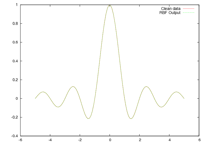
In this example, we use a RBF network with 10 kernels to approximate the sinc function on [-5.0,5.0] To make the life easier for the algorithm, we evenly spread the centers of the gaussians on [-5.0, 5.0].

The results are saved in 'example-003.data', the first column contains the x-position, the second column the result given by the trained RBF and the last column the value of sinc(x)

RBF learning the sinc function

Example 4 : Using a 2-2-3 MLP to learn three boolean functions : XOR, AND, OR

Example 5 : Using a 2-12-2 MLP to learn the Mackay-robot arm problem

In this example, we learn the two outputs (x,y) from the inputs (theta, phi) of the Mackay-robot arm dataset. For this we train a 2-12-2 MLP with a parametrized sigmoidal transfer function.

Learning the x-component

Learning the y-component

Example 6 : Finding the minimum of the Rosenbrock banana function

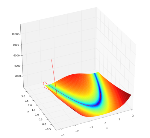
We use here UKF for parameter estimation to find the minimum of the Rosenbrock banana function :

Minimisation of the Rosenbrock banana function

Example 7 : Finding the parameters of a Lorentz attractor

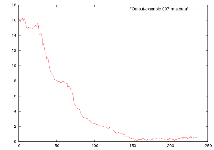
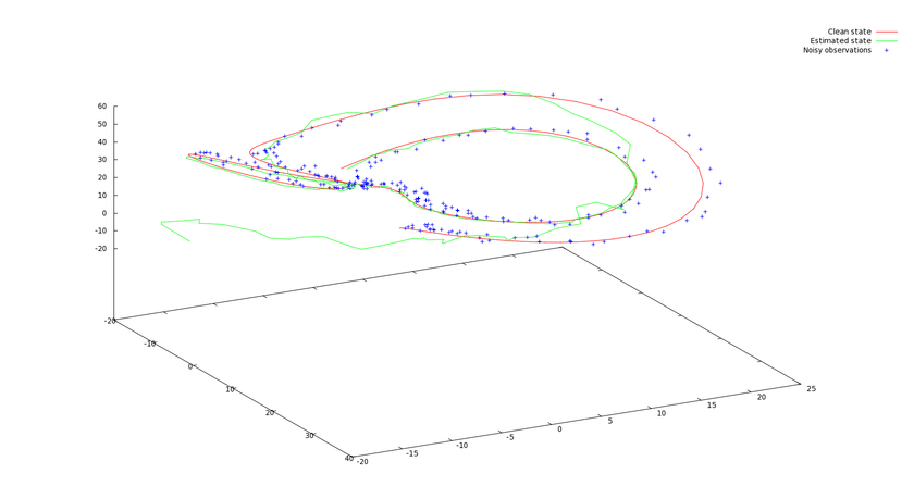
In this example, we try to find the parameters (initial condition, evolution parameters) of a noisy lorentz attractor. The dynamic of the lorentz attractor is defined by the three equations :

While observing a noisy trajectory of such a Lorentz attractor, the algorithm tries to find the current state and the evolution parameters . The samples we provide are .

To clearly see how UKF catches the true state, we initialized the estimated state of UKF to -15, -15 , -15

Learning RMS

Estimated state with the true state and its noisy observation